Cryogenic Heat Transfer: A Technical Engineering Reference

Jewlz Technologies
Aug 13
19 min read

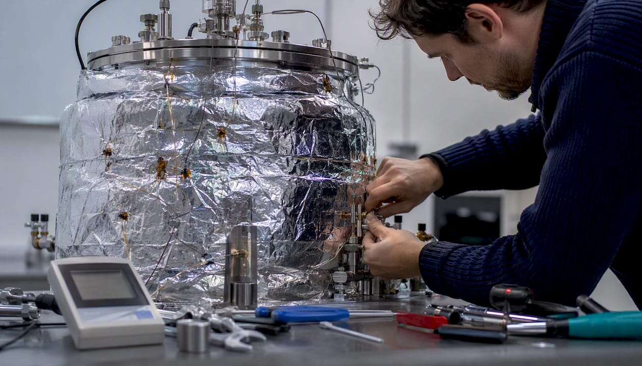
Cryogenic vessel with insulation and sensors

Cryogenic heat transfer covers heat exchange at temperatures below roughly −150 °C (−243 °F), where the physics depart sharply from room-temperature behavior. Thermal conductivity, specific heat, viscosity, and density all become strongly nonlinear functions of temperature. Two-phase and near-critical phenomena appear routinely, and radiative heat load from ambient surfaces can dominate if insulation is inadequate. Standard textbook correlations derived at 300 K often fail by large margins, so every credible cryogenic design starts with variable-property models and measured property data.

Four things to keep in mind before going further:

Variable properties invalidate room-temperature approximations. Thermal conductivity of copper, for example, peaks near 20 K and then drops sharply, a behavior that constant-property models miss entirely.
Two-phase phenomena and critical heat flux (CHF) set hard design limits. Boiling, condensation, and stratification are not edge cases in cryogenic systems; they are the normal operating regime for many components.
Vacuum plus multilayer insulation (MLI) is the primary defense against heat ingress. Radiation from a 300 K surface to a 20 K surface is the dominant heat load when conduction paths are already minimized.
Simulation requires variable-property CFD and a validated property database. NIST REFPROP is the standard source; pairing it with a solver that handles multiphase and conjugate heat transfer is non-negotiable.

Canonical starting points: Barron & Nellis, Cryogenic Heat Transfer for the full engineering treatment, the Clark chapter in Advances in Heat Transfer for a focused review, and the Thermalysis Toolkit from Jewlztech for applied variable-property conduction and convection calculations.

Key Takeaways

Cryogenic heat transfer requires variable-property modeling, two-phase awareness, and validated property data at every stage of design and simulation.

Point	Details
Variable properties are mandatory	Thermal conductivity and specific heat change by orders of magnitude below −150 °C; constant-property models produce unreliable results.
Two-phase and CHF set design limits	Boiling, stratification, and critical heat flux are normal operating conditions in cryogenic systems, not edge cases.
MLI and vacuum are the primary insulation strategy	Radiation from 300 K to 20 K dominates heat ingress; MLI below 10⁻⁵ torr is the standard mitigation.
Benchmark validation is non-negotiable	Stefan problem, pool-boiling curve, and slug-flow cases are practical minimums before trusting any cryogenic CFD model.
Thermalysis Toolkit for variable-property analysis	Jewlztech’s toolkit provides variable-property conduction and convection templates with a built-in property database for reproducible engineering calculations.

How cryogenic heat transfer differs from room-temperature conduction
Convection in cryogenic fluids: what changes and what stays the same
Two-phase flow, boiling, and critical heat flux in cryogenic systems
Why radiation dominates when insulation is inadequate
Material selection and thermophysical properties at low temperatures
How cryostat design minimizes heat ingress
Cryogenic heat exchangers and heat pipes: types and design cautions
Special regimes where standard models fail
A practical CFD workflow for cryogenic simulation
Instrumentation and experimental methods for cryogenic heat transfer
Applications and design red flags
Canonical equations, modelling assumptions, and where to go deeper
What cryogenic engineering actually demands in practice
The Thermalysis Toolkit handles the variable-property work that slows most cryogenic analyses
Sources

How cryogenic heat transfer differs from room-temperature conduction

Fourier’s law still governs conduction: q = −k(T) ∇T. The critical difference is that k is a function of temperature, not a constant. Across cryogenic ranges, k(T) can vary by an order of magnitude or more depending on the material, and the variation is often non-monotonic. Copper’s thermal conductivity rises steeply as temperature drops toward 20 K before falling again near absolute zero. Austenitic stainless steel follows a much flatter, lower curve. Treating either as a constant produces errors that are not small.

The governing equation for steady-state conduction with variable properties is:

∇ · [k(T) ∇T] = 0

For transient problems, add the volumetric heat capacity term: ρ c_p(T) ∂T/∂t = ∇ · [k(T) ∇T] + q̇

Both c_p and ρ are also temperature-dependent at cryogenic conditions, so the full variable-property form must be used. Barron & Nellis document this in detail and show where classical constant-property solutions diverge from measured results.

Material properties at cryogenic temperatures

Material	Typical use	Conductivity trend at cryo	Structural note
OFHC copper	Thermal links, heat straps	Very high; peaks near 20 K	Soft; not structural
Aluminum alloys (6061, 5083)	Heat exchangers, vessels	Good; decreases below 20 K	Ductile at cryo
Austenitic stainless steel (304, 316)	Pressure vessels, supports	Low (~10–15 W/m·K at 77 K)	Excellent toughness
G10/FR4 fiberglass composite	Structural supports, standoffs	Very low (~0.3 W/m·K)	Brittle below ~20 K
Invar	Low-expansion structures	Moderate	Near-zero thermal expansion

Thermal contraction is a separate concern. Aluminum contracts roughly twice as much as stainless steel between 300 K and 4 K, which introduces differential stress at joints and flanges. Design codes and material datasheets must be consulted for any structural component; never extrapolate room-temperature expansion coefficients to cryogenic ranges.

Hands holding cryogenic structural metal samples

Thermal contact resistance at cryogenic interfaces

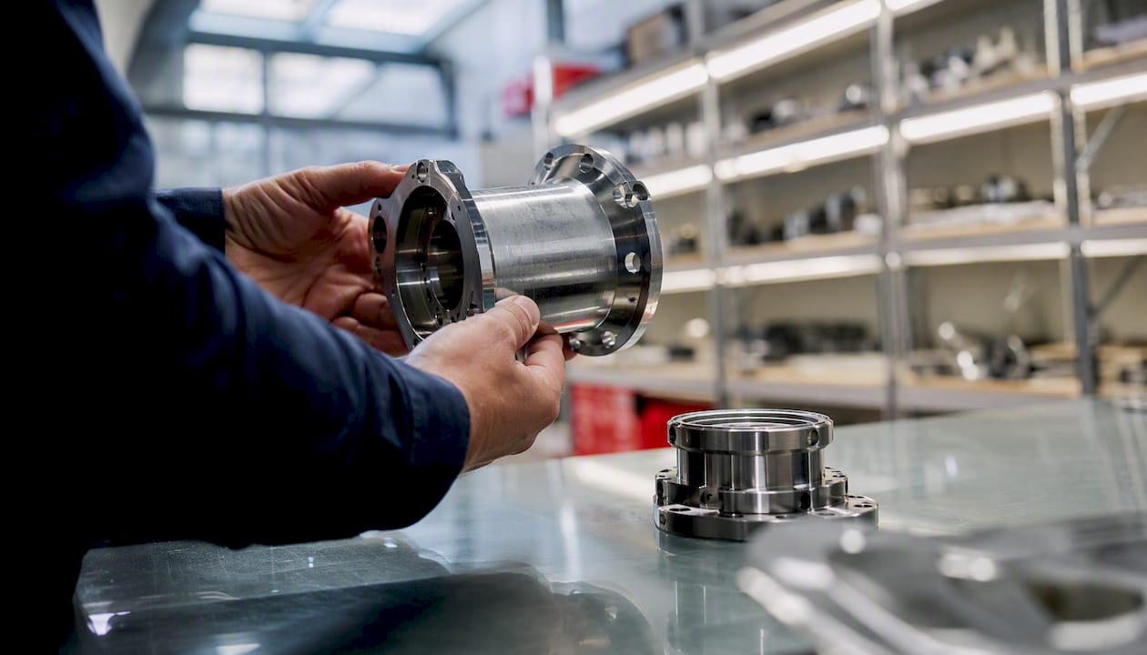
At cryogenic temperatures, the Kapitza conductance at solid-solid interfaces can dominate the total thermal resistance of an assembly. Kapitza conductance arises from acoustic mismatch between phonon populations across an interface and scales roughly as T³ at very low temperatures, meaning it drops sharply as you cool down. A joint that looks thermally negligible at 300 K can become the bottleneck at 4 K.

Practitioners handle this by designing joint preload carefully, inserting soft-metal interlayers (indium foil is common), and running in-situ calibration experiments to measure actual contact conductance rather than relying on literature estimates, which scatter widely. Barron & Nellis treat contact conductance at cryogenic interfaces as a first-class design variable, not an afterthought.

Pro Tip: When assembling cryogenic thermal joints, use a thin indium or annealed copper foil between mating surfaces, apply controlled and documented bolt torque, and instrument the joint with matched thermometers on both sides during the first cooldown. That in-situ measurement is worth more than any literature estimate.

Hands assembling cryogenic joint with indium foil

Convection in cryogenic fluids: what changes and what stays the same

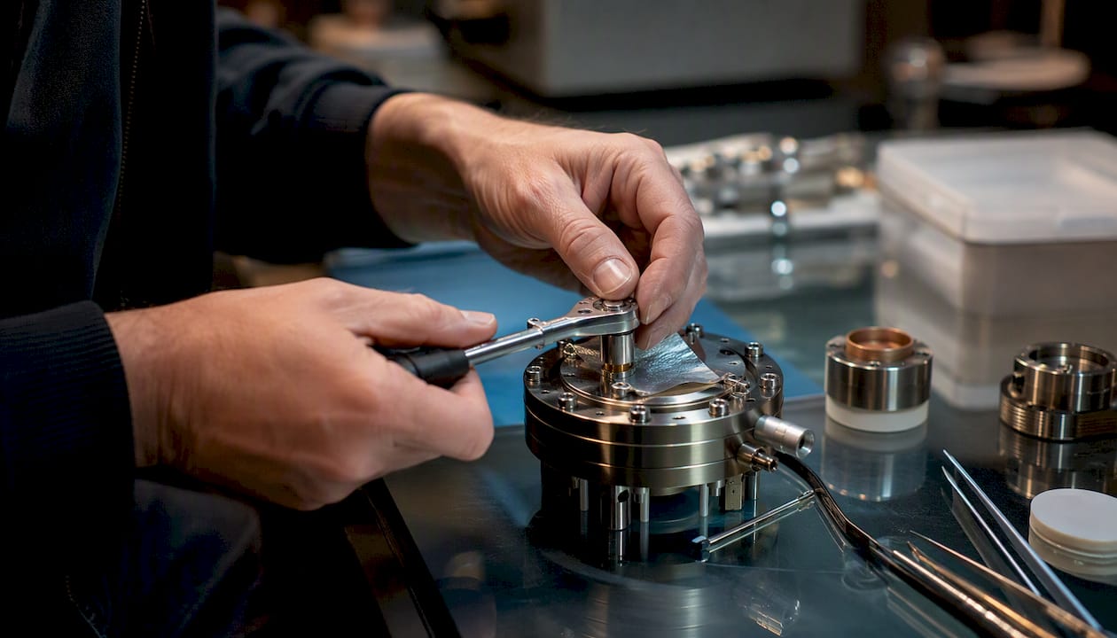
Convection in cryogenic gases and liquids follows the same governing equations as at room temperature: the Navier-Stokes equations coupled with the energy equation. What changes is that all fluid properties — density, viscosity, specific heat, and thermal conductivity — vary strongly with temperature and, near saturation, with phase. Reynolds, Prandtl, and Grashof numbers must be evaluated using local fluid properties, not bulk averages, or the resulting Nusselt number will be wrong.

The Dittus-Boelter correlation (Nu = 0.023 Re⁰·⁸ Pr^n) is a reasonable starting point for turbulent forced convection in cryogenic single-phase flows, but it was developed for moderate-property-variation conditions. When the ratio of wall-to-bulk viscosity or conductivity is large, property-correction factors (Sieder-Tate or Petukhov-type) are needed. Near the critical point of any working fluid, property variation becomes extreme and empirical correlations break down entirely; CFD with real-gas equations of state is the only reliable path.

Validation checklist for cryogenic convection models

Map fluid properties across the full temperature range. Pull data from NIST REFPROP and confirm that your solver interpolates them correctly at every grid cell, not just at inlet conditions.
Check sensitivity to property variation. Run the same case with constant properties at the bulk mean temperature and compare. If results differ by more than a few percent, variable-property treatment is mandatory.
Verify grid independence in the boundary layer. Cryogenic fluids often have low Prandtl numbers (LHe Pr ≈ 0.7; LH2 Pr ≈ 1.3), so the thermal and velocity boundary layers are similar in thickness. Confirm y⁺ targets are met for your turbulence model.
Check for near-critical behavior. If operating within roughly 10% of the critical pressure or temperature of your fluid, standard correlations are unreliable. Switch to a real-gas CFD model or a dedicated near-critical correlation.
Compare against a benchmark case. The LBL cryogenics notes provide sanity-check rules; use them before trusting a full simulation.
Natural convection check. In low-gravity or low-velocity regimes, Grashof number can be comparable to Re², meaning mixed convection. Evaluate Gr/Re² to determine whether natural convection is negligible.

Compressibility effects are generally small for cryogenic liquids but become relevant for cold helium gas at high flow velocities or in long transfer lines where pressure drop is significant. Near the critical point of helium (5.2 K, 2.27 bar), density fluctuations are large and the Boussinesq approximation fails; full compressible formulations are required.

Two-phase flow, boiling, and critical heat flux in cryogenic systems

Two-phase phenomena control heat transfer capacity and safety margins in most cryogenic systems. Boiling, condensation, stratification, and flash evaporation produce complex, often unsteady heat fluxes that single-phase models cannot capture. This is not a niche concern: any cryogenic storage vessel, transfer line, or heat exchanger operating near saturation will encounter two-phase behavior under normal conditions.

The boiling curve describes the progression from natural convection through nucleate boiling, transition boiling, and film boiling as wall superheat increases. CHF marks the point where the heat flux is high enough to sustain a vapor film on the heated surface, causing a sudden drop in heat transfer coefficient and a sharp rise in wall temperature. At cryogenic conditions, the latent heats of vaporization are small compared to room-temperature fluids (LN2 and LHe have relatively low latent heats of vaporization compared to room-temperature fluids, so the transition from nucleate to film boiling can happen at modest heat fluxes.) So the transition from nucleate to film boiling can happen at relatively modest heat fluxes. A design that ignores CHF in a cryogenic cooler is a design waiting to fail.

Stratification in storage tanks adds another layer of complexity. Density-driven separation of liquid and vapor phases creates temperature gradients that drive natural convection, which in turn affects boil-off rates and pressure buildup. In spacecraft tanks under microgravity, buoyancy-driven stratification disappears and thermocapillary effects take over — a regime discussed further in the special regimes section.

Modeling two-phase cryogenic flows

The Volume of Fluid (VOF) method and its combined Level Set variant (CLSVOF) are the most common interface-capturing approaches for sharp-interface two-phase problems. Phase-field methods offer thermodynamically consistent interface dynamics but at higher computational cost. For large tanks or simplified design calculations, homogeneous two-fluid models average the two phases and are much cheaper to run, at the cost of interface resolution.

The cryoFoam solver is an OpenFOAM-based research tool that implements CLSVOF with interfacial energy transport and tangential surface forces, specifically to reduce spurious velocities at cryogenic fluid interfaces and improve phase-change predictions for fluids like LH2, LOX, LN2, and LCH4. It validates against the Stefan solidification problem and pool-boiling benchmarks. Purdue and related benchmark studies supply slug-flow, bubble-dynamics, and tank boil-off cases that are practical minimums for validating any cryogenic two-phase solver.

Pro Tip: To avoid CHF in a cryogenic heater or heat exchanger: increase wetted surface area to lower local heat flux, encourage subcooling by pressurizing the liquid slightly above saturation, manage flow velocity to stay in the nucleate boiling regime, and use staged heat exchangers with control heaters to distribute the thermal load. Never rely on a single-point heat input in a cryogenic circuit.

Why radiation dominates when insulation is inadequate

Radiative heat flux scales with T⁴. A surface at 300 K radiating to one at 20 K produces a heat load that overwhelms conduction and convection through any reasonable gas gap if the vacuum is not maintained. The Stefan-Boltzmann law for two large parallel gray surfaces gives:

q_rad = σ (T₁⁴ − T₂⁴) / (1/ε₁ + 1/ε₂ − 1)

where σ = 5.67 × 10⁻⁸ W/m²·K⁴. For polished aluminum (ε ≈ 0.03) surfaces, this is manageable. For oxidized or contaminated surfaces (ε ≈ 0.1–0.3), the heat load rises by a factor of 3–10. View factor matters too: a cryostat with a poorly designed feedthrough that has a direct line of sight from a warm surface to the cold mass will leak heat at a rate that no amount of MLI on the main vessel can compensate.

MLI best practices

Layer count vs. compression. MLI performance degrades rapidly when layers are compressed. A 30-layer blanket compressed to half its design thickness can perform worse than a 10-layer blanket installed correctly. Target layer densities of roughly 20–30 layers per centimeter.
Low-emissivity foils. Double-aluminized Mylar (DAM) is standard. Crinkled foils reduce layer-to-layer contact and improve performance.
Guard rings and feedthrough shielding. Every penetration through an MLI blanket is a radiation leak. Design guard rings and reflective shields around all feedthroughs, supports, and instrumentation leads.
Vacuum quality target. MLI is effective only below roughly 10⁻³ torr; below 10⁻⁵ torr, residual gas conduction becomes negligible. At intermediate pressures, gas conduction through the blanket can exceed radiation.
Getter materials. In sealed cryostats, outgassing from materials at room temperature can degrade vacuum over time. Activated charcoal or zeolite getters cooled to cryogenic temperatures adsorb residual gas and maintain vacuum quality without active pumping.

For detailed vacuum insulation simulation approaches, the Jewlztech vacuum insulation panels guide covers practical modeling strategies.

Material selection and thermophysical properties at low temperatures

Materials behave differently at cryogenic temperatures, and the differences are large enough to drive design decisions. Thermal conductivity and specific heat can differ by orders of magnitude from room-temperature values, and thermal contraction introduces mechanical stress at every joint and interface. Picking a material for a cryogenic application means optimizing for both thermal and structural performance simultaneously.

Recommended materials and their typical roles:

OFHC copper. The go-to for thermal links and heat straps where maximum conductivity is needed. Purity matters: residual resistivity ratio (RRR) drives conductivity at low temperatures, and RRR > 100 is typical for cryogenic-grade copper.
Aluminum alloys (6061-T6, 5083). Good conductors, lightweight, and ductile at cryogenic temperatures. Common in heat exchangers and structural vessels where weight matters.
Austenitic stainless steels (304L, 316L). Low conductivity (which is an advantage for support structures), excellent toughness at low temperatures, and good weldability. The standard choice for pressure vessels and structural supports.
G10/FR4 fiberglass composite. Very low conductivity, making it ideal for support struts and standoffs where you want to minimize conductive heat leak. Becomes brittle below about 20 K; design accordingly.
Graphite composites. Used where very low thermal expansion and moderate conductivity are both needed, such as in telescope structures and some magnet support systems.

Never extrapolate room-temperature property data to cryogenic ranges. The Springer reference on low-temperature heat transfer documents that many standard solution approximations are invalid at low temperatures and recommends variable-property modeling throughout. NIST REFPROP and NIST’s cryogenic materials database are the authoritative sources for measured thermophysical property data; use them, not handbook tables from the 1970s.

Ductile-to-brittle transition is a real failure mode. Mild carbon steel, many polymers, and some aluminum alloys become brittle at cryogenic temperatures. ASME and other design codes specify minimum design temperatures for pressure-containing components; consult the relevant code edition and the material’s certified test report before specifying any structural part. The Hstar Schiller structural design guide provides a practical overview of these requirements.

How cryostat design minimizes heat ingress

The core strategy in cryostat design is straightforward: eliminate conduction paths, minimize radiation, and control boil-off. Every design decision flows from those three priorities. The USPAS cryostat design lecture notes provide a practical layout checklist that translates these priorities into hardware choices.

Design checklist:

Vacuum level. Target below 10⁻⁵ torr for the insulating vacuum space. Specify vacuum-compatible materials and processes for all internal components.
MLI selection. Choose layer count and foil type based on the temperature difference and available space. Install without compression.
Support geometry. Use thin-walled tubes or straps in materials with low thermal conductivity (G10, stainless steel thin-wall) rather than solid rods. Minimize cross-sectional area; maximize length.
Thermal intercepts. Attach intermediate-temperature heat sinks to support struts at one or more points along their length to intercept conducted heat before it reaches the cold mass.
Feedthrough routing. Route all electrical and instrumentation leads through thermal anchoring stages. Never run a copper wire directly from 300 K to 4 K without intermediate anchoring.
Piping and transfer lines. Use vacuum-jacketed transfer lines for any cryogen supply. Minimize the number of penetrations through the vacuum jacket.

Boil-off management depends on the application. Venting is simplest and acceptable for short-duration or low-cost operations. Recondensing with a pulse-tube or Gifford-McMahon cryocooler is the right choice for long-duration or closed-loop systems where cryogen resupply is impractical. Reliquefaction plants are used at large-scale facilities (particle accelerators, MRI manufacturing) where the cryogen volume justifies the capital cost.

Pro Tip: Place thermal intercepts at every intermediate temperature stage available in your system, typically at 77 K (liquid nitrogen shield) and 20 K (second stage of a two-stage cryocooler). Each intercept cuts the conduction load to the next colder stage by the ratio of temperature differences, which compounds quickly across multiple stages.

Cryogenic heat exchangers and heat pipes: types and design cautions

Plate-fin, brazed aluminum, perforated-plate, and regenerator designs are the workhorses of cryogenic heat exchange. Heat pipes extend the toolkit by moving large heat loads passively through two-phase operation. Each geometry has a specific niche.

Plate-fin heat exchangers. High surface area per unit volume, excellent effectiveness, and well-suited to multi-stream service. Standard in air separation plants and hydrogen liquefaction. Aluminum brazing limits operating temperature to above roughly 4 K; below that, stainless or copper construction is needed.
Brazed plate heat exchangers. Compact and effective for LN2 service (~77 K). Less flexible for multi-stream service than plate-fin but easier to source commercially.
Perforated-plate (stacked-disc) exchangers. Used where fouling or particulate contamination is a concern, since the open geometry is easier to clean. Common in helium liquefiers.
Regenerators. Essential in Stirling, Gifford-McMahon, and pulse-tube cryocoolers. The regenerator matrix (stainless mesh, lead spheres, or rare-earth materials at very low temperatures) stores and releases heat cyclically. Rare-earth materials like Er₃Ni are used below 10 K because their specific heat peaks in that range, which stainless steel and lead do not.

Working fluid selection is driven by temperature and application. A recent review confirms that liquid nitrogen (LN2, ~77 K) is the most widely used cryogen because of low cost and ready availability. Liquid helium (LHe, ~4.2 K) is chosen when temperatures near absolute zero are required. Liquid oxygen (LOX) and liquid methane (LCH4) are the propellants of choice in modern launch vehicles, and their heat-transfer behavior in engine cooling circuits and tank systems is an active research area. Cautions: LOX is a strong oxidizer and requires scrupulously clean systems; LCH4 can form ice plugs if moisture is present; LHe requires careful pressure management to avoid solidification.

Frost mitigation in heat exchangers exposed to humid ambient air requires either vacuum jacketing or purging with dry gas. Fin spacing choices matter: tighter fins increase surface area but are more susceptible to blockage by frost or ice. For exchangers that must operate in non-vacuum environments, wider fin spacing and periodic warm-up cycles are standard practice.

Special regimes where standard models fail

Superfluid helium (He II), microgravity two-phase behavior, and thermocapillary-dominated flows each invalidate assumptions that work everywhere else. Treating any of these with a standard single-phase or conventional two-phase model produces results that are qualitatively wrong, not just quantitatively off.

He II (superfluid helium below 2.17 K). Below the lambda point, helium transitions to a superfluid state with effectively zero viscosity and anomalously high thermal conductivity. Heat transport occurs via second sound — a temperature wave propagating through the superfluid component — rather than through diffusion. The Gorter-Mellink mutual friction term governs heat flux at higher heat loads, and the effective thermal conductivity of He II is a nonlinear function of heat flux, not a material constant. Kapitza conductance at He II interfaces is also distinct from normal-fluid behavior. Barron & Nellis cover He II heat transport in detail; for experimental work, the relevant literature on second-sound attenuation and Kapitza resistance must be consulted directly.

Microgravity two-phase behavior. In spacecraft propellant tanks, buoyancy-driven stratification and natural convection disappear under microgravity. Liquid-vapor interfaces are governed by surface tension rather than gravity, leading to complex slosh dynamics and unpredictable vapor pocket locations. Thermocapillary (Marangoni) convection driven by surface tension gradients along the interface can dominate heat and mass transfer. Predicting propellant behavior during engine restart requires dedicated microgravity models and, ideally, experimental data from drop-tower or orbital tests.

Thermocapillary flows. At small scales or under strong temperature gradients, surface tension gradients drive Marangoni convection that can be stronger than buoyancy-driven flow even at normal gravity. This is relevant in thin-film evaporators, micro-channel heat exchangers, and any cryogenic system where the characteristic length scale is small. Standard CFD codes require explicit Marangoni stress boundary conditions at the interface to capture this correctly.

A practical CFD workflow for cryogenic simulation

Credible cryogenic modeling needs four things: variable-property capability, robust multiphase handling, validated property data, and documented benchmark comparison. Skip any one of them and the results will mislead rather than inform.

Recommended workflow

Step	Action	Tool / source
1. Property sourcing	Pull k(T), c_p(T), ρ(T), μ(T), σ(T) for all fluids and solids	NIST REFPROP, NIST cryo materials DB
2. Solver selection	Single-phase conjugate HT: any capable FVM solver; two-phase: VOF/CLSVOF or two-fluid	OpenFOAM/cryoFoam, ANSYS Fluent
3. Mesh and time step	Resolve boundary layers (y⁺ target per turbulence model); time step controlled by CFL criterion for VOF	Solver-specific meshing tools
4. Boundary and initial conditions	Set realistic wall temperatures, heat fluxes, and inlet profiles; initialize two-phase fraction carefully	CFD boundary conditions guide
5. Convergence and sensitivity	Monitor residuals, energy balance, and key output quantities; run property-sensitivity sweep	Solver post-processing
6. Benchmark validation	Compare against Stefan problem, pool-boiling curve, slug-flow data, and tank boil-off	Purdue benchmark cases

cryoFoam is the current state of the art for non-isothermal two-phase interface capture in cryogenic fluids, implementing CLSVOF with interfacial energy transport and tangential surface forces. ANSYS Fluent supports phase-change modeling through its mixture and Eulerian multiphase models and is widely used in industry for cryogenic heat exchanger and storage vessel analysis. For variable-property conduction and convection analyses that do not require full multiphase CFD, the Thermalysis Toolkit from Jewlztech provides a focused, applied engineering environment with built-in property tables and conjugate heat transfer templates.

For a broader look at solver options, the Jewlztech SimScale alternatives guide covers the practical trade-offs across solver classes.

Pro Tip: Archive your complete case: mesh files, property tables, boundary condition scripts, and a short validation report with experimental comparison. Reproducibility is increasingly expected in published cryogenic simulation work, and having the archive ready saves significant time when reviewers or collaborators ask for it.

Instrumentation and experimental methods for cryogenic heat transfer

Accurate cryogenic experiments depend on minimizing parasitic heating, selecting the right sensors, and building a quantified uncertainty budget. A CFD validation campaign is only as good as the experimental data it validates against, and cryogenic measurements are notoriously easy to corrupt with poorly managed heat leaks.

Key instrumentation:

Cernox thermometers. The standard choice for 0.1–420 K. Low magnetoresistance makes them suitable for magnet environments. Calibration is required; factory calibrations are available but in-situ calibration against a reference standard is better practice.
Silicon diode thermometers. Good sensitivity across 1.4–500 K; more sensitive to magnetic fields than Cernox. Common in non-magnet environments.
Vapor-pressure thermometry. Absolute accuracy for specific fluids (LHe, LN2, LH2) at saturation; useful as a primary reference for calibrating other sensors.
Heat flux sensors. Thin-film Gardon gauges or differential thermopile sensors rated for cryogenic temperatures. Placement and thermal anchoring of leads are critical.
Capacitance level gauges. Reliable for measuring liquid levels in cryogenic vessels; immune to the electromagnetic noise that affects some other sensor types.
Pressure transducers. Must be rated for cryogenic service; diaphragm-type sensors with remote sensing lines are common to keep the transducer body at a warmer temperature.

Pro Tip: Thermal-anchor every instrumentation lead at each temperature stage it passes through. A single un-anchored 36-AWG copper wire running from 300 K to 4 K carries roughly 1–2 mW of parasitic heat, which is enough to swamp the signal in a precision calorimetry experiment. Use phosphor-bronze or manganin wire for leads where low conductivity matters, and document every thermal anchor in your uncertainty budget.

Uncertainty analysis should follow GUM (Guide to the Expression of Uncertainty in Measurement) methodology. When submitting results for CFD validation, include the full uncertainty budget alongside the data so that modelers can assess whether discrepancies are within experimental scatter or represent genuine model error.

Applications and design red flags

Different applications emphasize different failure modes. Knowing which failure mode dominates in your application is the fastest way to focus design effort.

Spacecraft propellant systems. Mass minimization drives every decision. MLI layer count is optimized against launch mass; support structures are designed to the minimum cross-section that survives launch loads. Under microgravity, liquid-vapor interface location is uncertain, so propellant management devices (PMDs) and surface-tension-driven screens are used to ensure vapor-free liquid delivery to the engine. Design checks: verify MLI installation quality and vacuum integrity before integration; model microgravity slosh with a dedicated solver; confirm PMD performance across the full range of fill fractions. For broader context on heat transfer applications in aerospace and other sectors, Jewlztech’s reference guide covers the key design considerations.
Superconducting magnets (MRI, accelerators, fusion). The dominant concern is quench: a local transition from superconducting to normal-conducting state that releases stored magnetic energy as heat. He II conductance through the winding pack determines how quickly heat spreads and whether the quench is benign or destructive. Thermal intercepts on current leads are critical; a poorly designed current lead can deliver more heat to the cold mass than the entire radiation load. Design checks: calculate He II heat transport capacity through the winding cross-section; verify current lead intercept temperatures; confirm quench protection heater coverage.
LNG and cryogenic storage vessels. Boil-off rate is the primary performance metric. Stratification during filling creates a warm layer at the top of the tank that drives pressure buildup and rollover risk. Venting strategy must account for the full range of fill levels and ambient heat loads. Design checks: calculate steady-state boil-off rate from insulation performance; model stratification during filling and hold; verify pressure relief valve sizing against worst-case heat ingress.

Red flags to watch for in any cryogenic system:

Unexpected rapid boil-off, which usually indicates an insulation failure, vacuum loss, or an unaccounted conduction path.
Brittle fracture indications at joints or welds, which suggest a material specification error or an unanticipated temperature excursion.
Large unexplained thermal gradients across a component that should be nearly isothermal, pointing to a contact resistance problem or a blocked flow path.
Persistent mismatch between model predictions and experimental measurements that exceeds the stated uncertainty budget, which means either the model physics are wrong or the experiment has an unquantified heat leak.

Canonical equations, modelling assumptions, and where to go deeper

The equations below are the starting points for cryogenic thermal analysis. Each needs modification or careful re-evaluation at low temperatures.

Fourier conduction: q = −k(T) ∇T. Use k(T) from measured databases; never use a room-temperature constant.
Nusselt correlation (Dittus-Boelter type): Nu = C Re^m Pr^n. Evaluate Re and Pr at local fluid temperature; apply property-correction factors when wall-to-bulk property ratios are large.
Boiling curve / CHF: Use fluid-specific correlations (Kutateladze, Zuber, or experimentally derived) with cryogenic fluid properties. Room-temperature CHF correlations do not transfer.
Stefan problem (phase change): ρ L dX/dt = k ∂T/∂x at the moving interface, where L is latent heat and X is interface position. Latent heat values for cryogens are small; interface motion can be fast.
Radiative exchange: q_rad = σ (T₁⁴ − T₂⁴) / (1/ε₁ + 1/ε₂ − 1) for parallel gray surfaces. View factor must be calculated for real geometries.

Standard assumptions and when they fail

Constant properties. Fails at any cryogenic temperature for any material or fluid. Use variable-property models throughout.
Single-phase flow. Fails whenever the fluid is near saturation, which is the normal operating condition for most cryogenic storage and transfer systems.
Negligible radiation. Fails whenever vacuum insulation is imperfect or when warm surfaces have direct view factors to cold surfaces.
Boussinesq approximation for natural convection. Fails near critical points and in microgravity.
Incompressible flow. Fails for cold helium gas at high velocities or near the critical point.

The Springer Heat Transfer at Low Temperatures reference documents these failure modes systematically. For a practical heat transfer modeling guide covering canonical equations and methods, Jewlztech’s engineering reference is a useful companion.

What cryogenic engineering actually demands in practice

The textbook treatment of cryogenic heat transfer is thorough, but it tends to present each mechanism in isolation: conduction here, boiling there, radiation in its own chapter. Real cryogenic systems couple all of them simultaneously, and the failure modes almost always live at the interfaces between those mechanisms, not in the middle of any one of them.

The trade-off that comes up most often is simulation fidelity versus development time. A full multiphase CFD campaign with real-gas properties and interface-capturing numerics can take weeks to set up and validate.

Three checks before committing to a design approach:

Validate first, then refine. Run the simplest benchmark case your solver can handle before building the full model. If it cannot reproduce the Stefan problem or a canonical pool-boiling curve, the full model will not be trustworthy either.
Prefer staged designs. A system with thermal intercepts at 77 K and 20 K is more forgiving than one that tries to jump from 300 K to 4 K in a single stage. Staged designs also make instrumentation and troubleshooting easier.
Plan instrumentation before the design is frozen. Adding a thermometer port or a heat-flux sensor access point after fabrication is expensive. Decide where the critical measurement points are during the design phase and build access in from the start.

The Thermalysis Toolkit handles the variable-property work that slows most cryogenic analyses

Variable-property conduction and convection calculations are where most cryogenic engineering workflows stall. Setting up a full CFD campaign for every design iteration is impractical; using constant-property approximations produces results that cannot be trusted. The Thermalysis Toolkit from Jewlztech sits in that gap: a focused, downloadable Excel-based engineering toolkit that handles variable-property thermal analysis for conduction, convection, and radiation without requiring a full CFD setup.

The toolkit includes a built-in material property database, conjugate heat transfer templates, and exportable case files that feed directly into CFD preprocessing workflows. For engineers running the benchmark cases described in the modeling section, it provides a reproducible starting point with documented assumptions and property sources. The variable-property input structure means you can pull data directly from NIST and run parametric sweeps across temperature ranges relevant to LN2, LHe, or LCH4 service without rebuilding the calculation from scratch each time.

If you are working through the benchmark validation workflow described above or need a defensible variable-property analysis for a design review, start with the Thermalysis Toolkit to establish your baseline before scaling up to full multiphase CFD.