
CFD Boundary Conditions: A Practical Engineer's Guide


CFD boundary conditions are mathematical constraints applied at the edges of a computational domain that close the governing Navier–Stokes and continuity equations, making the problem solvable. Without them, the system of partial differential equations has infinitely many solutions. Get them wrong and you get divergence, mass imbalance, or results that look plausible but are physically meaningless.
The main types every engineer needs to know:
Inlet: velocity inlet, mass-flow inlet, total pressure inlet
Outlet: pressure outlet, outflow/zero-gradient
Wall: no-slip, slip, moving wall, roughness
Symmetry / axisymmetric: mirror planes, axisymmetric no-swirl
Periodic / cyclic: translational and rotational repeating geometries
Far-field / open: freestream, pressure far-field, non-reflecting
Thermal: fixed temperature, heat flux, convective film coefficient, conjugate
Pro Tip: The single most common failure mode is over-specification: setting both velocity and pressure at the same patch. Before debugging residuals, check whether you have prescribed more constraints than the governing equations require at any one boundary.
Table of Contents
Why do CFD boundary conditions make or break your simulation?
How do Dirichlet, Neumann, and Robin conditions map to solver labels?
When should you use symmetry or periodic boundary conditions?
What are far-field and open boundary conditions for external flows?
How do you choose boundary conditions and avoid common pitfalls?
Translating physical measurements into solver boundary conditions
Why do CFD boundary conditions make or break your simulation?
Every CFD solver discretizes the Navier–Stokes and continuity equations into a large algebraic system. Boundary conditions supply the values or gradients at the domain edges that anchor that system. Without physically consistent BCs, the matrix is either under-determined (infinitely many solutions) or over-determined (no solution at all).
The conceptual split is simple. A Dirichlet condition prescribes the variable itself: φ = φ_wall. A Neumann condition prescribes its normal derivative: ∂φ/∂n = q. Most CFD boundary conditions reduce to one of these two, or a combination called Robin. The choice at each patch determines which rows of the linear system are fixed by data and which are solved.
Incorrect BCs produce recognizable failure signatures:
Non-convergence: residuals stall or oscillate without settling
Mass imbalance: net flux through the domain is nonzero
Wrong flow direction: reversed inlet or outlet flow from the first iteration
Spurious recirculation: unphysical vortices near boundaries that pollute the interior
The governing principle is that BCs must be physically realistic, provide a well-posed problem, and be compatible across every equation being solved simultaneously. A BC that satisfies the momentum equation but violates the energy equation will cause the energy residual to diverge even when velocity looks fine.
How do Dirichlet, Neumann, and Robin conditions map to solver labels?
Every solver UI name is a wrapper around one of three mathematical operators. Recognizing which operator a label enforces is the fastest way to diagnose a convergence problem, because it tells you exactly which matrix row is being constrained and how.
Solver labels map to underlying math as follows:
Mathematical type | Typical solver label(s) | Practical example |
Dirichlet (fixed value) | Velocity inlet, fixed temperature wall | u = 5 m/s; T = 300 K |
Neumann (fixed gradient) | Outflow, zero-gradient outlet, symmetry | ∂u/∂n = 0; ∂T/∂n = 0 |
Robin (value + gradient) | Convective wall, film coefficient | h(T − T∞) = −k ∂T/∂n |
Mixed / composite | Pressure outlet (p fixed, velocity extrapolated) | p = atmospheric pressure; ∂u/∂n = 0 |
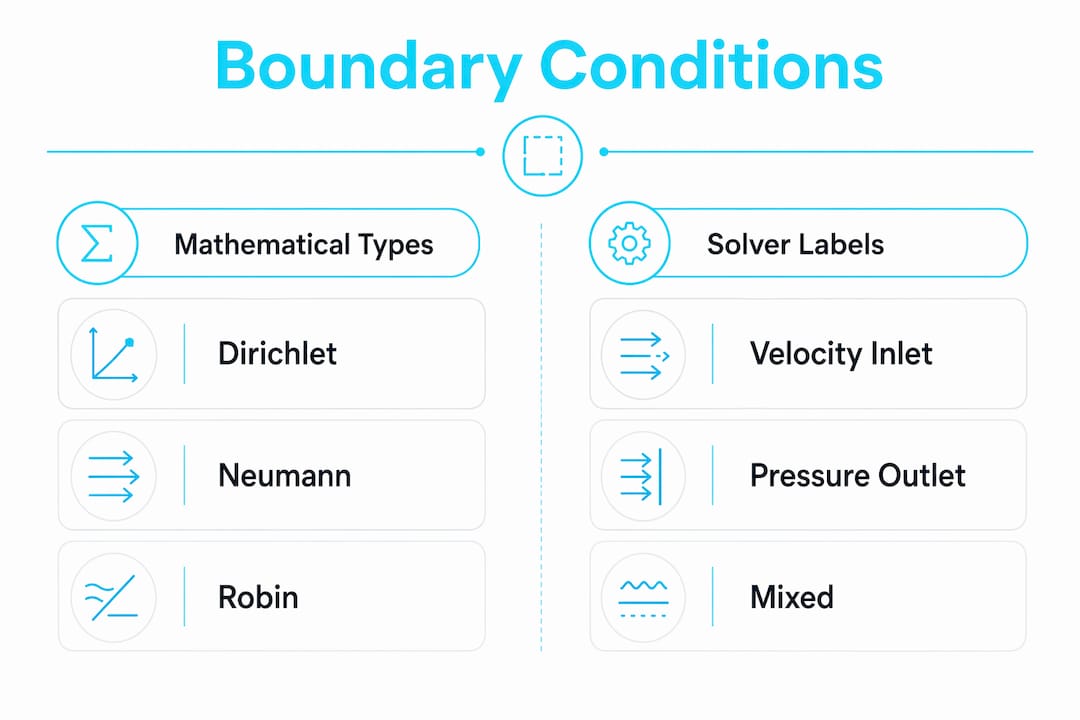
A velocity inlet sets u, v, w as Dirichlet values. A pressure outlet fixes static pressure (Dirichlet on p) while extrapolating velocity (Neumann on u). A symmetry plane enforces zero normal velocity and zero normal gradient for all other variables — pure Neumann. A convective wall applies a Robin condition linking surface temperature to a film coefficient and ambient temperature.
Pro Tip: Before trusting a solver’s default, open the documentation and confirm whether it applies a value or a gradient operator. “Pressure outlet” in one solver may extrapolate turbulent quantities from the interior; in another it may reset them to specified values. The UI name alone does not tell you.
What are the right inlet boundary conditions to use?
Choose the inlet BC that matches the quantity you actually measured or control. If you have a flow meter, use mass-flow inlet. If you have a velocity probe, use velocity inlet. If you are modeling a compressible nozzle fed by a plenum, use total pressure / total conditions.
Common inlet options and when each fits:
Velocity inlet: use when you have a measured or specified velocity magnitude and direction; works for incompressible and mildly compressible flows
Mass-flow inlet: preferred when the mass flow rate is the controlled variable (e.g., a pump or fan curve); avoids the need to convert to velocity when density varies
Total pressure inlet: correct for compressible or high-speed flows where stagnation conditions are known; the solver derives static pressure and velocity from the Mach number internally
Fully developed profile: import or specify a parabolic (laminar) or 1/7th-power-law (turbulent) profile when the upstream duct is long enough that the flow is already developed
For turbulence, inlet turbulence specification requires at minimum a turbulence intensity (I) and a length scale or hydraulic diameter. Typical values: I = 1–5% for duct flows, I = 0.1% for free-stream external flows. The solver uses these to derive k and ε (or k and ω) internally. Supplying k and ε directly is more accurate when you have measured turbulence data.
Pro Tip: Fitting a measured velocity profile to a parabolic or power-law function and importing it as a UDF or expression reduces startup transients dramatically. A uniform inlet profile on a short domain forces the solver to develop the boundary layer inside the domain, which consumes mesh and distorts near-inlet results.
Which outlet boundary conditions avoid instability?
Use a pressure-based outlet when the downstream environment pressure is known. Use an outflow or zero-gradient condition only when the flow is genuinely fully developed at the exit and the solver cannot determine pressure from the interior alone.
Outlet options and their constraints:
Pressure outlet: sets static gauge pressure at the exit; the solver extrapolates velocity; most robust choice for incompressible flows; requires a backflow specification for turbulence and temperature
Outflow / zero-gradient: assumes ∂φ/∂n = 0 for all variables; inappropriate for compressible flows or cases with strong pressure gradients at the exit; the solver extrapolates interior values
Supersonic / unknown outlet: used when the flow exits supersonically; no downstream information propagates upstream, so no BC on pressure is needed
A practical rule of thumb: place the outlet at least 8–10 hydraulic diameters downstream of any geometry feature that generates wakes or recirculation. Closer placement forces the BC to interact with unresolved flow structures and causes pressure-outlet instability. For external flows, 15–20 body lengths downstream is a common starting point.
Pro Tip: Always specify backflow turbulence intensity and temperature at a pressure outlet, even if you expect no reverse flow. If backflow occurs during iteration and those values are unset, the solver uses defaults that can spike residuals and trigger divergence. A backflow turbulence intensity of 5% and a temperature equal to the inlet value is a safe starting point.
How should you specify wall boundary conditions?
Walls enforce the momentum and thermal conditions that govern near-wall behavior. The choice of wall specification depends on mesh resolution and the physics you need to capture.
Wall types and when to use them:
No-slip (stationary wall): u = v = w = 0 at the wall; correct for viscous flows; requires either a fine mesh to resolve the viscous sublayer or a wall function to bridge it
Slip wall: zero normal velocity, zero shear stress; appropriate for inviscid approximations or free-surface boundaries where viscous effects are negligible
Moving wall: prescribes a wall velocity (translational or rotational); used for rotating machinery, conveyor problems, or Couette flow setups
Rough wall: adds a roughness height (ks) that modifies the log-law intercept; critical for pipe flow, terrain, and heat exchanger surfaces
The y+ value governs which near-wall approach is valid. Wall treatment choice is often the dominant source of thermal error in conjugate problems:
y+ < 1: resolve the viscous sublayer directly; required for low-Reynolds turbulence models (k-ω SST in low-Re mode, Spalart-Allmaras); gives accurate wall shear and heat flux
y+ 30–300: use wall functions (standard or enhanced); reduces cell count significantly; acceptable for bulk flow predictions where near-wall detail is secondary
Pro Tip: When specifying roughness, use the equivalent sand-grain roughness height (ks), not the arithmetic mean roughness (Ra). The two are related but not equal — using Ra directly in a wall-function roughness model underestimates friction by a factor that varies with surface type.
When should you use symmetry or periodic boundary conditions?

Use symmetry or axisymmetric boundaries when both the geometry and the flow field are mirrored. Use periodic boundaries when the geometry and solution repeat spatially, either translationally or rotationally.
Correct use cases:
Symmetry plane: geometry has a mirror plane AND the flow has no swirl or asymmetric loading; halves the domain instantly
Axisymmetric (2D): geometry is a solid of revolution with no circumferential variation; reduces a 3D problem to 2D
Translational periodicity: flow through a bank of tubes or a heat sink fin array where the fin pitch repeats
Rotational periodicity: a single blade passage in a turbomachine representing the full annulus
Periodic and rotational periodic boundaries enforce identical solution variables across paired faces. The mesh on mating faces must match node-for-node, or the solver must interpolate, which introduces error. For heat sink fins or blade passages, symmetry and periodic BCs can reduce cell counts dramatically while preserving thermal fidelity. See the Jewlztech post on COMSOL simulation alternatives for a discussion of how different solvers handle cyclic BC pairing.
Pro Tip: In transient simulations with rotating periodic boundaries, check whether your solver requires a phase-shift specification for non-integer blade counts. Missing the phase shift produces a solution that looks converged but has an unphysical circumferential discontinuity at the periodic interface.
What are far-field and open boundary conditions for external flows?
For external aerodynamics and other unbounded flows, far-field boundaries mimic an infinite domain. The goal is to let disturbances leave the domain without reflecting back into the solution.
Far-field options:
Freestream / velocity inlet (far-field): sets uniform velocity and direction far from the body; suitable for incompressible external flows; domain must be large enough that the BC does not constrain the wake
Pressure far-field: used in compressible solvers; specifies Mach number, static pressure, and temperature; the solver applies Riemann invariants to allow waves to exit without reflection
Non-reflecting / radiation BCs: absorb outgoing pressure or acoustic waves; used in aeroacoustics and unsteady compressible simulations where pressure waves must not bounce off the outlet
Domain size rules of thumb for external flows: place the inlet 5–10 body lengths upstream, the outlet 15–20 body lengths downstream, and lateral boundaries 10–15 body lengths from the body centerline. These distances reduce the boundary’s influence on the near-body pressure field to an acceptable level for most engineering accuracy targets.
Pro Tip: For unsteady simulations with vortex shedding or acoustic sources, add a sponge layer or damping zone in the last 10–20% of the domain before the outlet. The sponge gradually increases artificial dissipation, absorbing outgoing disturbances before they reach the boundary and reflect.
How do you set thermal boundary conditions correctly?
Thermal BCs follow the same Dirichlet/Neumann/Robin framework as flow BCs. The choice must match the heat-transfer model being solved.
Thermal BC types and example applications:
Fixed temperature (Dirichlet): T = T_wall; use when the wall temperature is controlled or measured (e.g., a thermostatically controlled surface, a phase-change boundary)
Heat flux (Neumann): q = q_wall [W/m²]; use when the power input is specified (e.g., an electric heater with a known wattage per unit area)
Convective film coefficient (Robin): q = h(T_wall − T∞); use when the external convection coefficient is known from correlations or measurements; typical h values are 5–25 W/m²K for natural convection in air and 50–500 W/m²K for forced convection in air
Conjugate heat transfer (CHT): solve conduction in the solid simultaneously with convection in the fluid; use when the wall temperature distribution is unknown and the thermal resistance of the solid matters
Inaccurate wall thermal BCs — wrong h values or neglected contact resistance — are often the largest source of error in conjugate simulations. If you are assembling multiple parts with interfaces, always account for contact resistance rather than assuming perfect thermal contact. For practical thermal design scenarios, the Jewlztech guide on heat transfer techniques covers when CHT is worth the added solver cost versus applying an estimated h.
Pro Tip: Never apply both a fixed temperature and a heat flux to the same wall patch. It over-specifies the thermal problem at that face, which is the thermal equivalent of setting both velocity and pressure at a flow boundary. Pick one: either you know the temperature or you know the flux, not both.
How do you choose boundary conditions and avoid common pitfalls?
The one-line rule: prescribe the BC that matches the quantity you can actually measure or control at that boundary, and prescribe it only once per variable per patch.
Decision checklist
You have measured velocity: use velocity inlet; specify turbulence intensity and hydraulic diameter
You have measured mass flow: use mass-flow inlet; avoids density-conversion errors in variable-density flows
You know only the upstream pressure: use total pressure inlet; let the solver derive velocity
You know the downstream environment pressure: use pressure outlet; set gauge pressure to the known value
Flow is fully developed at the exit: use outflow/zero-gradient; confirm the outlet is far enough downstream
Compressible flow: use total conditions at inlet and pressure far-field or supersonic outlet; never use outflow BC
Common errors
Over-specification: setting both velocity and pressure at the same patch; the discrete system becomes inconsistent and diverges
Under-specification: leaving a patch with no BC; the solver uses a default that may not match your physics
Inconsistent turbulence BCs: specifying turbulence intensity at the inlet but leaving the outlet turbulence unset; backflow during iteration imports unphysical turbulence levels
Outlet too close to geometry: placing the outlet within 2–3 diameters of a bend or obstruction; the zero-gradient assumption is violated and pressure-outlet instability follows
Mismatched periodic faces: mesh node counts differ on paired faces; the solver interpolates across the interface and introduces artificial diffusion
Troubleshooting steps when BCs are suspect
Check global mass balance: net inlet flux minus net outlet flux should be less than 0.1% of the inlet flux
Examine residuals by equation: a residual that spikes for one equation (e.g., energy) while others converge points to a BC inconsistency in that equation
Enable monitoring probes at boundary patches: watch velocity and pressure at the outlet face to detect reverse flow or pressure locking
Simplify BCs to find the offending patch: replace complex profiles with uniform values, disable turbulence models temporarily, and reintroduce complexity one patch at a time
Three worked examples with boundary condition assignments
Example 1: Turbulent flow through a rectangular duct
Setup: air at 20°C, Re ≈ 50,000, duct cross-section 0.1 m × 0.1 m, length 1 m.
Inlet: velocity inlet, u = 7.5 m/s, turbulence intensity I = 5%, hydraulic diameter D_h = 0.1 m
Outlet: pressure outlet, gauge pressure = 0 Pa, backflow I = 5%, backflow T = 293 K
Walls: no-slip, adiabatic; target y+ 30–100 with standard wall functions
Validation: compare computed friction factor to the Moody chart at Re = 50,000; mass flow at outlet should match inlet within 0.1%
Gotcha: placing the outlet at exactly 1 m (10 D_h) is borderline. If residuals oscillate, extend to 15 D_h and recheck.
Example 2: Flat-plate boundary layer (laminar to turbulent)
Setup: flat plate in air, L = 0.5 m, U∞ = 10 m/s, Re_L ≈ 340,000 (transitional).
Inlet (left face): velocity inlet, u = 10 m/s uniform, I = 0.1% (low freestream turbulence)
Top face: symmetry (zero normal velocity, zero normal gradient) — acts as a freestream boundary
Plate (bottom face): no-slip, adiabatic; y+ < 1 to resolve the viscous sublayer
Outlet: pressure outlet, gauge pressure = 0 Pa
Validation: compare wall shear stress distribution to the Blasius solution for the laminar portion (x < x_crit); the Blasius profile gives C_f = 0.664 Re_x^(−0.5)
Gotcha: a uniform inlet profile is acceptable here because the plate leading edge defines the boundary-layer origin. Do not use a developed profile — it would impose an incorrect initial condition.
Example 3: Fully developed channel flow with periodic BCs
Setup: 2D channel, height H = 0.02 m, target Re_H = 10,000; use periodic BCs to avoid specifying a developed profile.
Inlet / outlet faces: translational periodic pair; the solver enforces identical velocity and turbulence across the pair with a specified pressure drop or mass flow driving force
Walls: no-slip; y+ < 1 for DNS-quality or y+ 30–100 for RANS with wall functions
Alternative: if the solver does not support periodic with a pressure gradient, use a mass-flow inlet and an outflow BC on a domain at least 60 H long
Gotcha: when using a periodic pressure-drop formulation, confirm the solver adds the mean pressure gradient as a source term in the momentum equation rather than applying it as a BC. Some solvers require this to be enabled explicitly.
Pro Tip: For all three examples, run a mesh sensitivity study by refining the near-wall layer by a factor of two and comparing the target output (friction factor, wall shear, Nusselt number). If the result changes by more than 5%, the mesh is not yet independent of resolution.
Step-by-step debugging when BCs cause divergence
The fastest path to a working simulation is staged isolation: simplify BCs to the minimum physically meaningful set, confirm convergence, then add complexity.
Disable turbulence models temporarily. Run laminar first. If the laminar case converges and the turbulent case does not, the problem is in turbulence BC specification or wall treatment, not the flow BCs.
Switch from transient to steady-state. Transient simulations amplify BC errors at every time step. A steady-state run with the same BCs reveals whether the problem is a BC issue or a time-stepping issue.
Reduce under-relaxation factors. For pressure-velocity coupling, drop under-relaxation to 0.3/0.5 (pressure/momentum). If the simulation stabilizes, the BCs are likely correct but the initial condition is far from the solution.
Inspect boundary fluxes. Most solvers can report the net flux through each named patch. A patch showing a flux in the wrong direction (e.g., outflow at an inlet) signals a BC or initialization error.
Extend the outlet domain. If the pressure outlet shows reverse flow from iteration 1, the outlet is too close to a geometry feature. Extend by 5 D_h and restart.
Change outlet type. If a pressure outlet is unstable, try an outflow/zero-gradient BC temporarily. If the simulation converges, the issue is the pressure value specified at the outlet, not the flow physics.
Verify mesh near critical boundaries. A y+ value far outside the target range (e.g., y+ = 500 when using a low-Re model expecting y+ < 1) causes wall-function errors that propagate into the interior and destabilize the solution.
Pro Tip: Build complexity in layers: first verify mass conservation with a coarse mesh and simple BCs, then refine the mesh, then add turbulence, then add heat transfer. Each layer has a known correct answer to check against. Skipping layers and debugging a fully coupled multiphysics model from scratch wastes hours.
Translating physical measurements into solver boundary conditions
The core translation: what you measure in the lab or field maps directly to what the solver needs at each patch.
Measured / known quantity | Solver BC to set | Example settings | Notes |
Duct velocity (Pitot tube) | Velocity inlet | u = measured value; I = 3–5%; D_h = duct diameter | Fit a profile if traverse data is available |
Mass flow rate (flow meter) | Mass-flow inlet | ṁ = measured value; I = 3–5% | Preferred for variable-density flows |
Upstream stagnation pressure | Total pressure inlet | p_0 = measured; T_0 = measured | Required for compressible flows |
Downstream static pressure | Pressure outlet | p_gauge = p_measured − p_atm | Set backflow T and I to avoid divergence |
Wall heat load (power supply) | Heat flux BC | q = Power / Area [W/m²] | Verify area matches the heated patch area |
External convection coefficient | Film coefficient (Robin) | h = 5–25 W/m²K (natural conv.); 50–500 W/m²K (forced conv.) | Use CHT if wall temperature distribution matters |
Repeating geometry | Periodic / cyclic BC | Match mesh on paired faces; specify pressure drop or mass flow | Confirm solver supports pressure-gradient source term |
For sensitivity testing, vary inlet turbulence intensity across its plausible range (e.g., 1% to 10% for a duct) and record the change in the target output (Nusselt number, pressure drop). If the output shifts by more than the measurement uncertainty, the simulation result is sensitive to a quantity you may not know precisely. Report that sensitivity alongside the result. The same test applies to outlet gauge pressure: a ±5% variation in specified pressure should produce a proportionally small change in interior velocity if the outlet is correctly placed.
Industrial pipe flow setups are a practical case where measured flow rates and pipe sizing directly determine which inlet BC is appropriate and what turbulence parameters to supply. Similarly, common installation mistakes in piping systems often translate into incorrect flow boundary assumptions in CFD models.
Pro Tip: Document every BC assumption in a simulation log: the source of each value (measured, estimated, literature), the date, and the uncertainty. When a result is questioned six months later, that log is the difference between a defensible answer and a guess.
Key Takeaways
Correct CFD boundary conditions require matching each solver BC to a physically measured or controlled quantity, avoiding over-specification, and verifying mass balance before trusting any result.
Point | Details |
Match BC to measurement | Use velocity inlet for probe data, mass-flow inlet for flow meter data, pressure outlet for known downstream pressure. |
Avoid over-specification | Never prescribe both velocity and pressure at the same patch; it makes the discrete system inconsistent and causes divergence. |
Check mass balance first | Net inlet flux minus net outlet flux should be within 0.1% before interpreting any flow or thermal result. |
Use symmetry/periodic to cut cost | Periodic and symmetry BCs can reduce cell count dramatically for repeating geometries while preserving thermal fidelity. |
Jewlztech thermal toolkit | Jewlztech’s simulation toolkit supports CFD and thermal BC setup with a built-in property database for conduction, convection, and radiation workflows. |
Why engineers keep getting boundary conditions wrong
The gap between textbook BC theory and what actually happens in a solver is wider than most courses admit. Students learn Dirichlet and Neumann conditions in a PDE class, then open a commercial solver and find labels like “pressure outlet” or “outflow” with no clear indication of which mathematical operator is being applied. The result is that engineers often pick BCs by intuition or by copying a tutorial case without checking whether the tutorial’s geometry, Reynolds number, or flow regime matches their own.
The deeper problem is that translating physical reality into algebraic constraints is genuinely hard. A real duct has a fan upstream with a known pressure rise, a flow meter reading mass flow, and a thermocouple at the wall. None of those map cleanly to a single BC type without a judgment call. Engineers who skip the judgment call and use defaults are not being lazy; they often do not know the defaults exist or what they assume.
Two things that actually help: first, always run a sensitivity study on the BCs you are least certain about before reporting results. Second, keep a simulation log that records the source and uncertainty of every BC value. Both habits take ten minutes and save hours of post-hoc debugging.
Useful sources and further reading
The following references support the technical content in this article and are worth bookmarking for solver-specific details:
Notes on CFD: General Principles, Chapter 4 — the clearest concise treatment of what makes a BC set well-posed; read this before opening any solver
CFD.University: How to Implement Boundary Conditions — practical mapping of mathematical types to solver labels; good for students moving from theory to practice
Bakker Lecture 6: Boundary Conditions — covers turbulence inlet specification and outflow BC limitations in a format useful for graduate coursework
Autodesk CFD Help: Physical Boundaries (2024) — solver-specific documentation on wall treatment, y+ guidance, and symmetry/periodic setup
Wikipedia: Boundary Conditions in Computational Fluid Dynamics — a useful overview of BC types with links to deeper mathematical treatments
Always consult your solver’s own manual for the exact default assumptions behind each named BC. Defaults vary between solvers and versions, and a default that is correct for one flow regime may be wrong for another. For students looking for accessible tools to practice CFD and thermal simulation setup, the Jewlztech engineering software guide covers options across experience levels.
Jewlztech makes thermal and CFD simulation more accessible
Setting up boundary conditions correctly is only half the challenge. The other half is having a simulation environment that gives you direct control over those settings without a steep learning curve or a five-figure software license.

Jewlztech’s Thermalysis Toolkit is built for exactly the workflows this article covers: conduction, convection, and radiation analysis with support for variable material properties, a wide temperature range, and multiple heat-transfer modes. The toolkit includes a built-in property database so you are not hunting for material values when you are trying to set a thermal BC. It runs as a downloadable Excel-based tool, which means no cloud dependency and no per-seat enterprise pricing. Engineers who need to run thermal simulations without committing to a full commercial CFD platform will find it a practical starting point. Visit the Thermalysis Toolkit page to review the features and start a subscription.
Recommended
Comments