
Thermal Contact Resistance: Engineering Guide for Professionals


Thermal contact resistance (TCR) is the temperature drop across an interface divided by the heat flow through it: R_c = ΔT / Q, with units of K/W for a specific joint or m²·K/W when normalized by contact area. Its inverse is thermal contact conductance, h_c = 1/R_c. Both quantities appear in every heat-transfer network where two solids meet imperfectly, and ignoring them in high-flux paths is one of the most reliable ways to underpredict junction temperatures.
A few things to know before going further:
When it matters most: metal-to-metal joints in power electronics, heat sinks, bolted flanges, and cryogenic assemblies. For low-flux applications with large bulk resistances, TCR is often negligible.
Typical range: experimental literature places most metal-metal contacts between 5×10⁻⁶ and 5×10⁻⁴ m²·K/W, corresponding to conductance values of roughly 2,000 to 200,000 W/m²·K. A single order-of-magnitude error here can shift a junction temperature prediction by tens of degrees.
Measure first when accuracy is required: analytical models are useful for scoping, but ASTM-style steady-state cut-bar tests remain the standard for defensible data. Jewlztech’s Thermalysis Toolkit supports rapid sensitivity sweeps when you need to bound the problem before committing to a test campaign.
Table of Contents
What is thermal contact resistance, and how does it fit into heat-transfer equations?
What parameters actually control contact resistance in practice?
Which analytical models should you use to estimate contact resistance?
How can you reduce contact resistance during design and assembly?
How do you quantify and report measurement uncertainty in TCR experiments?
Worked example: computing R_c and h_c from a steady-state test
Using simulation and engineering toolchains to predict contact resistance
Run parametric contact resistance studies with the Thermalysis Toolkit
What is thermal contact resistance, and how does it fit into heat-transfer equations?
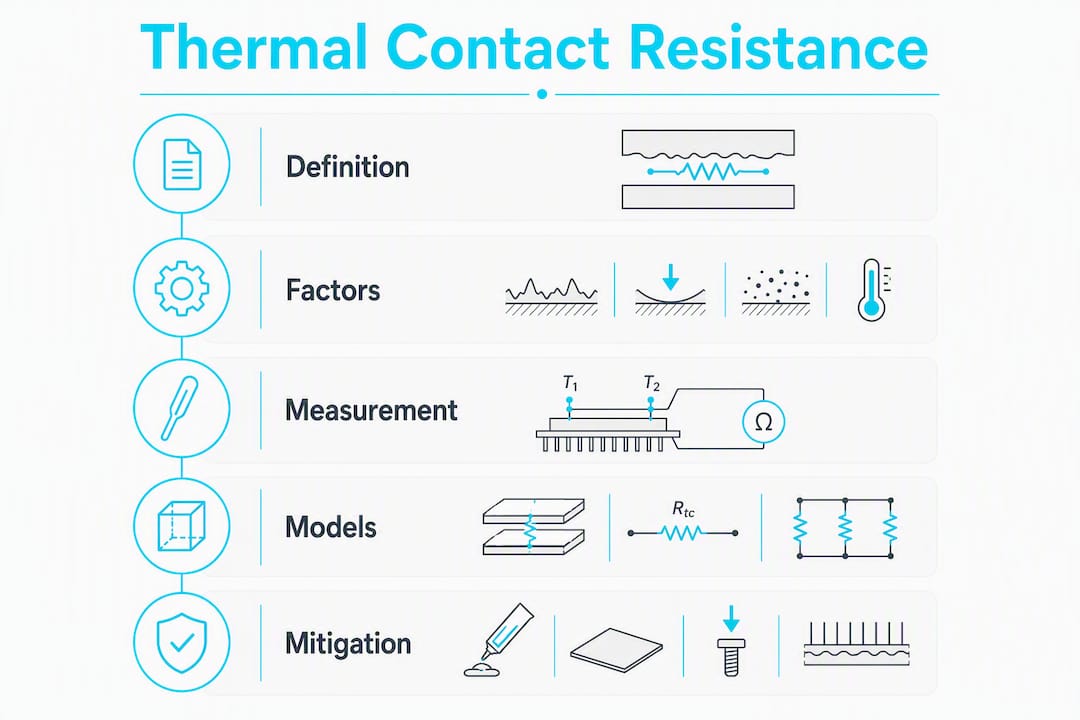
Thermal contact resistance is formally defined as the ratio of the temperature drop at an interface to the average heat flow across it. In equation form:
R_c = (T₁ − T₂) / Q
where T₁ and T₂ are temperatures on either side of the interface and Q is the steady-state heat flow in watts. Contact conductance is simply h_c = 1/R_c (W/K for a whole joint) or, when normalized by the apparent contact area A:
R_c’’ = ΔT / (Q/A) [m²·K/W] h_c’’ = 1/R_c’’ [W/m²·K]
The area-normalized form is preferred when comparing material pairs or surface treatments across different specimen sizes. Use the whole-joint form (K/W) when you are building a lumped thermal network for a specific assembly.
Placing TCR in a 1D conduction model
Inserting contact resistance into a series thermal network is straightforward:
Identify each solid layer and compute its bulk resistance: R_bulk = L / (k·A), where L is thickness, k is thermal conductivity, and A is cross-sectional area.
Place R_c between the two bulk terms: R_total = R₁ + R_c + R₂.
Compute the total temperature drop: ΔT_total = Q · R_total.
Check whether R_c is significant relative to R₁ + R₂. If R_c < 5% of R_total, you can often lump it into a boundary condition without meaningful error.
In finite-element models, TCR appears as a contact conductance boundary condition applied at the interface node pair, not as a material property. Getting that placement right matters: applying it as a bulk material layer instead introduces geometry-dependent errors that scale with mesh refinement.
Why does thermal contact resistance exist at all?
No machined surface is perfectly flat. At the microscale, every surface is a landscape of peaks (asperities) and valleys. When two surfaces are pressed together, contact occurs only at those asperity tips, and the real contact area is a small fraction of the apparent (geometric) area. Heat trying to cross the interface must squeeze through those microcontact spots, producing a constriction in the heat flux lines that raises local thermal resistance. That constriction effect is the physical core of TCR.
“In vacuum, conduction through micro-contact spots is the dominant heat-transfer mode at an interface; models typically separate geometrical, mechanical, and thermal components — and researchers identify three distinct TCR regions for nonconforming rough contacts, determined by the ratio of macro- to micro-thermal resistances.” ASME Heat Transfer
Macro vs. micro resistance components
Practitioners separate TCR into two components in series:
Macro-scale resistance arises from waviness and flatness errors. Even a surface with low roughness can have a gentle bow that concentrates contact at the center and leaves the perimeter nearly unloaded. This macro component dominates when the wavelength of surface deviation is much larger than the asperity scale.
Micro-scale resistance comes from roughness: the individual asperity contacts that carry the actual heat flux. Each microcontact acts as a constriction, and the aggregate of thousands of them sets the micro-component of TCR.
Both components sit in series, so the one with the higher value controls the total. Polishing a surface to sub-micron roughness while ignoring flatness can leave macro resistance unchanged and produce almost no improvement in conductance.
Heat transfer modes across the interface
Three mechanisms carry heat across the gap between asperity contacts:
Conduction through microcontacts — the dominant path in most engineering applications.
Conduction through the interstitial medium — air, gas, grease, or a solid thermal interface material (TIM) filling the gap. The thermal conductivity of the gap filler and the gap geometry (related to the Knudsen number for thin gas layers) determine how much this path contributes.
Radiation across the gap — Thermopedia notes this is negligible below roughly 700 K for most engineering contacts, though it becomes relevant in high-temperature furnace assemblies or space hardware.
Visualize it this way: heat flux lines converge from a broad cross-section in the bulk material, squeeze through the asperity contact spots, then fan back out. The gap regions between asperities either conduct through the filler or are effectively dead zones in vacuum.
Asperity deformation matters too. At low contact pressures, asperities deform elastically and spring back when unloaded. At higher pressures, plastic deformation flattens them permanently, increasing real contact area and reducing TCR. Whether a given interface is in the elastic or plastic regime depends on material hardness, yield strength, and the applied load — which is why hardness appears in most TCR models.

What parameters actually control contact resistance in practice?
Contact conductance depends on material thermophysical and mechanical properties, surface roughness, waviness, flatness, interstitial media, and contact pressure. That list is not equally weighted. Here is how the variables rank in practice:
Contact pressure: the single strongest lever. Higher load increases real contact area nonlinearly. Doubling pressure does not double conductance, but the trend is consistent and predictable. Light loads combined with low temperatures correlate with the highest resistance values.
Surface roughness (RMS) and mean surface slope: finer finishes reduce the asperity constriction component. Mean slope matters as much as RMS amplitude because it sets the angle at which asperities meet and deform.
Waviness and flatness: macro-scale deviations that set how uniformly load distributes across the interface. A bowed plate pressed against a flat one concentrates stress at the center; the perimeter carries almost no load and contributes little to conductance.
Interstitial medium: filling the gap with a material of higher thermal conductivity than air (k_air ≈ 0.026 W/m·K at room temperature) directly reduces the gap-conduction resistance. Thermal greases typically reach 1–10 W/m·K; metallic foils can exceed 100 W/m·K.
Material hardness: softer materials deform more readily under load, increasing real contact area. Copper-to-copper contacts generally show lower TCR than steel-to-steel at the same nominal pressure.
Surface chemistry and contamination: oxide layers and films can create a high-resistance barrier that mechanical preload alone cannot penetrate. A thin aluminum oxide layer, for example, has thermal conductivity roughly 30 W/m·K — not terrible in isolation, but its presence as a discontinuous film at microcontacts adds a series resistance that shifts the effective conductance by a factor of two or more in some cases.
Mean junction temperature: thermal expansion changes contact geometry, and higher temperatures can soften asperities or alter oxide thickness. For high-precision designs, thermal expansion and thermal stresses can change contact geometry and must be considered.
Environmental pressure: in vacuum, the interstitial gas path disappears entirely, and TCR rises sharply compared to ambient conditions. This is why space hardware and vacuum furnace assemblies require metallic interlayers or bonded joints.
Pro Tip: Identify the three variables with the highest sensitivity for your specific application before running a full parametric study. For most ambient-pressure metal-metal joints, that trio is contact pressure, surface roughness, and interstitial material conductivity. Sweep those first; the others are second-order.
Which analytical models should you use to estimate contact resistance?
No single model covers the full range of contact conditions. Reviews confirm that analytical models apply only to limiting cases and that many experimental points fall in transition ranges between regimes, which is why experimental calibration remains essential even when a good model is available.
The major model families
Cooper–Mikic–Yovanovich (CMY): the most widely cited semi-empirical correlation for conforming rough contacts. CMY expresses contact conductance as a function of surface roughness (σ), mean asperity slope (m), material hardness (H), contact pressure (P), and bulk conductivity (k_s). The core relation takes the form:
h_c / (k_s · m/σ) = C · (P/H)^n
where C and n are empirical constants (approximately 1.25 and 0.95 for plastic deformation). CMY assumes circular microcontacts, a Gaussian height distribution, and either fully plastic or fully elastic asperity deformation. It performs well for conforming surfaces under moderate to high loads.
Greenwood–Williamson (GW) approaches: originally developed for tribology, GW models treat asperities as spherical caps with a statistical height distribution. They are well-suited for elastic contact regimes and provide the foundation for many subsequent TCR extensions. The key output is the number and size distribution of microcontact spots as a function of load.
Holm-type constriction models: Holm’s classical result for a single circular constriction gives the spreading resistance as R_spread = 1/(2·k·a), where a is the contact spot radius. Summing over all microcontacts gives the aggregate micro-resistance. This approach is transparent and easy to implement but requires an independent estimate of contact spot size and density.
Scale-analysis (Bahrami/Majumdar-style): Bahrami’s scale-analysis model introduces a nondimensional parameter equal to the ratio of macro- to micro-thermal resistances, which identifies three TCR regions and compares well to experimental data across a wide range of nonconforming rough contacts. This approach is particularly useful when you cannot classify your contact as purely conforming or nonconforming.
Choosing a model: a practical sequence
Characterize the geometry: is the contact conforming (flat-on-flat) or nonconforming (curved-on-flat, sphere-on-flat)? Conforming contacts suit CMY; nonconforming contacts need GW or scale-analysis.
Estimate the contact pressure and hardness ratio (P/H): if P/H < 0.01, elastic models apply; above ~0.1, plastic deformation dominates; in between, use a mixed or scale-analysis approach.
Check whether interstitial gas matters: if the gap conductance from air is comparable to the microcontact conductance, use a model that includes the interstitial term (extended CMY or Yovanovich’s gas-gap models).
Select the limiting-case model that matches your regime and compute a first estimate.
Validate against at least two experimental data points at different loads. If the model diverges by more than 30%, recalibrate the empirical constants or switch models.
How do you measure contact resistance reliably?
Steady-state vs. transient methods
Steady-state methods (cut-bar, guarded-hot-plate variants) apply a known, stable heat flux through a stack that includes the interface of interest. Temperature sensors on either side of the interface measure ΔT; Q is determined from a calibrated heater or a reference material with known conductivity. The contact resistance is then R_c = ΔT/Q after subtracting bulk contributions. These methods are well-suited for high-accuracy work and are the basis for most published TCR databases.
Transient methods (laser flash analysis, transient heat-flux sensors) apply a short thermal pulse and measure the temperature response. Laser flash analysis is fast (seconds per measurement) and works well for thin samples, but extracting contact resistance requires careful modeling of the pulse propagation through the stack. Transient methods are better for screening and ranking than for absolute accuracy.
Method | Principle | Instrumentation | Test Duration | Bulk Sensitivity | Best Environment |
Cut-bar (steady-state) | Steady heat flux, ΔT across interface | Thermocouples/RTDs, calibrated heater | 30–120 min | High (must subtract) | Vacuum or ambient |
Guarded hot plate | Controlled guard heater eliminates lateral losses | Guard heater, precision thermometry | 60 min | High | Ambient |
Laser flash | Thermal pulse, rear-face temperature response | Laser, IR detector, reference samples | 1–5 min | Moderate | Ambient or vacuum |
Transient heat-flux sensor | Step heat flux, sensor response | Thin-film sensor, fast DAQ | 1–30 min | Low | Ambient |
Instrumentation checklist
Temperature sensors: type-T or type-K thermocouples for ambient tests; platinum RTDs (PT100/PT1000) for higher accuracy. Place sensors as close to the interface as geometry allows, and account for the distance correction when computing ΔT at the interface.
Heat-flux measurement: use a calibrated reference bar with known k, or a direct heat-flux sensor. Calibrate the heater power independently.
Data acquisition: sample at a rate that captures thermal equilibrium clearly. For steady-state tests, confirm equilibrium by checking that sensor readings drift less than 0.1 K over 10 minutes.
Clamping hardware: use a load cell or calibrated torque wrench to measure actual contact force, not just applied torque. Torque-to-force conversion depends on thread friction and varies by 20–30% without lubrication.
Sample preparation and reporting
Clean contact surfaces with isopropyl alcohol or acetone before testing. For oxide-sensitive materials (aluminum, copper), consider a light abrasive pass followed by immediate assembly to minimize re-oxidation. Report nominal contact area, measured surface roughness (Ra or Rq), cleaning method, clamping force, and ambient conditions alongside the TCR value.
Experimental test rigs must subtract bulk resistance to avoid overestimating contact resistance. The standard approach: measure the total stack resistance, then measure each bulk layer separately (or compute from k and geometry), and subtract. Skipping this step systematically biases TCR estimates high.
Relevant standards for thermal interface material testing include ASTM D5470 (steady-state heat flux method for TIMs) and ASTM E1530 (guarded heat flow meter). For broader thermal conductivity testing, ASTM E1461 covers laser flash analysis.
Pro Tip: Always run tests at a minimum of three contact pressure levels. A single-point measurement tells you nothing about the pressure sensitivity, which is often the most important design variable. Plotting R_c vs. P on a log-log scale reveals the regime and helps you extrapolate to operating conditions.
What are typical values of thermal contact resistance?
Knowing whether your measured or estimated TCR is physically plausible is the first sanity check. The table below gives representative ranges from experimental literature.
Contact Type | Typical R_c’’ (m²·K/W) | Notes |
Soldered / diffusion-bonded joint | ~10⁻⁷ to 10⁻⁶ | Near-ideal; limited by bulk solder conductivity |
Metal foil interlayer (indium, copper) | ~10⁻⁶ to 10⁻⁵ | Effective in vacuum; conductivity of foil sets floor |
Pressed metal-metal with TIM (grease) | ~10⁻⁵ to 10⁻⁴ | Highly sensitive to grease thickness and coverage |
Pressed metal-metal, no TIM, ambient | ~10⁻⁵ to 5×10⁻⁴ | Strongly pressure- and roughness-dependent |
Pressed metal-metal, vacuum, light load | ~10⁻⁴ to 10⁻³ | Gas-gap path eliminated; asperity conduction only |
Rough or contaminated surface, low load | Can exceed 10⁻³ | Oxide films and poor contact dominate |
The 5×10⁻⁶ to 5×10⁻⁴ m²·K/W range cited in experimental literature covers the middle of this spread — well-prepared metal surfaces under reasonable loads. Values outside that range are real but indicate either exceptional preparation (low end) or poor surface condition or vacuum environment (high end).
Caveat: a single TCR measurement at one load and one surface condition is nearly meaningless for design. Surface condition, contact pressure, and the presence or absence of interstitial material each shift the value by one to two orders of magnitude. Always characterize the sensitivity, not just the point estimate.
How can you reduce contact resistance during design and assembly?
The options range from free (clean and torque correctly) to expensive but permanent (bonding or soldering). Choosing the right one depends on your thermal budget, reworkability requirements, and operating environment.
Higher clamping preload: the cheapest first step. Increasing bolt torque raises contact pressure and reduces TCR nonlinearly. Verify with a load cell rather than relying on torque alone; thread friction variation makes torque an unreliable proxy for force.
Surface finishing (lapping, polishing): reduces the micro-scale roughness component. Effective when macro flatness is already controlled. Lapping to Ra < 0.4 µm typically yields a measurable improvement for metal-metal contacts; going finer than Ra 0.1 µm produces diminishing returns unless the macro component is also addressed.
Compliant TIMs (greases, phase-change materials, pads): fill the gap with a higher-conductivity medium. Thermal greases are the most common choice in electronics cooling. Their effectiveness depends on bond-line thickness — thinner is better, but too thin causes pump-out under thermal cycling. Phase-change materials address pump-out but add cost.
Metallic interlayers (indium foil, copper foil, solder): highly effective, especially in vacuum or cryogenic applications where greases are impractical. Coatings such as indium improve conductance in vacuum applications by providing a soft, conforming metallic path that mechanical preload alone cannot replicate. Indium’s low hardness means it deforms plastically at modest loads, maximizing real contact area.
Bonding and soldering: the lowest achievable TCR for a permanent joint. Eliminates the interface resistance almost entirely, replacing it with the bulk resistance of the bond layer. The trade-off is reworkability: a soldered joint is not field-serviceable without reflowing.
Coatings: electroplated nickel or silver on contact surfaces reduces oxide growth and improves conductance. Watch for galvanic corrosion when dissimilar metals are involved — a nickel-plated aluminum surface in contact with bare copper can corrode at the interface over time.
For heat transfer applications in power electronics, the typical design sequence is: clean surfaces, apply a well-characterized TIM, torque to a measured load, and verify with a thermal resistance measurement at operating temperature.
Pro Tip: For vacuum or cryogenic applications, skip greases entirely. They outgas, pump out, and lose effectiveness at low temperatures. Metallic interlayers (indium is the standard choice) or welded/bonded joints are the correct solution. Budget for the added assembly complexity.
How do you quantify and report measurement uncertainty in TCR experiments?
A TCR value without an uncertainty estimate is not a result — it is a guess with a decimal point. Measurement best practice requires explicit subtraction of bulk contributions and reporting of an uncertainty budget; without this, contact resistance estimates are systematically biased high.
Common error sources
The dominant contributors in a typical steady-state cut-bar test:
Bulk resistance inclusion: failure to subtract the bulk terms of the sample layers. This is the most common and most consequential error.
Sensor placement error: thermocouples placed even 1 mm away from the interface introduce a ΔT offset proportional to the local heat flux and material conductivity.
Lateral heat losses: radiation and convection from the sample sides reduce the actual heat flow through the interface below the heater power. Vacuum enclosures or guard heaters mitigate this.
Uneven contact pressure: non-uniform bolt patterns or warped surfaces create pressure gradients that make the measured ΔT a spatial average over a non-uniform contact.
Temperature drift: if the system has not reached true steady state, the measured ΔT includes a transient component. Confirm equilibrium before recording data.
Calibration uncertainty: thermocouple accuracy is typically ±1–2 K without individual calibration; RTDs with NIST-traceable calibration can reach ±0.1 K.
Best-practice reporting checklist
Report sample geometry: dimensions, material, and measured bulk thermal conductivity (not just the nominal value from a datasheet).
Document surface preparation: cleaning method, roughness measurement (Ra or Rq, instrument used), and time between preparation and assembly.
State clamping method and measured contact force (not just applied torque).
List sensor types, locations relative to the interface, and calibration traceability.
Report raw total resistance and the bulk-subtracted contact resistance separately.
Provide an uncertainty budget identifying the top three contributors and their estimated magnitudes.
State the number of repeat tests and report mean ± expanded uncertainty at 95% confidence, not a single value.
For a typical metal-metal steady-state test, sensor placement and bulk subtraction together often account for 60–80% of the total uncertainty. Addressing those two sources first gives the largest return on calibration effort.
Worked example: computing R_c and h_c from a steady-state test
Problem statement
Two aluminum plates (k = 160 W/m·K) are pressed together with a contact area A = 25 cm² (0.0025 m²). A steady-state test measures:
Total temperature drop across the stack: ΔT_total = 12.5 K
Heat flow: Q = 50 W
Each plate is 10 mm thick
Step-by-step calculation
Compute total thermal resistance: R_total = ΔT_total / Q = 12.5 / 50 = 0.25 K/W
Compute bulk resistance for each plate: R_bulk = L / (k · A) = 0.010 / (160 × 0.0025) = 0.025 K/W per plate Two plates: R_bulk_total = 2 × 0.025 = 0.050 K/W
Isolate contact resistance: R_c = R_total − R_bulk_total = 0.25 − 0.050 = the difference between total and bulk resistances, representing the contact resistance.
Normalize by area: R_c’’ = R_c ÷ A = 0.20 ÷ 0.0025 = a normalized contact resistance value reflecting resistance per unit area.
Convert to contact conductance: h_c = 1 / R_c = 1 / 0.20 = 5 W/K (whole joint) h_c’’ = 1 / R_c’’ = the contact conductance calculated as the inverse of normalized resistance.
Unit consistency check: R_c’’ [m²·K/W] × Q/A [W/m²] = ΔT [K]. Plugging in: 5×10⁻⁴ × (50/0.0025) = 5×10⁻⁴ × 20,000 = 10 K. The contact accounts for 10 K of the 12.5 K total drop. ✓
Interpretation and sensitivity
The contact term dominates: 10 K out of 12.5 K (80%) comes from the interface, not the bulk aluminum. This is a high-resistance case — R_c’’ = 5×10⁻⁴ m²·K/W sits at the upper end of the typical range for metal-metal contacts, suggesting either a light contact load, a rough surface, or a contaminated interface.
Adding a thermal grease with k = 3 W/m·K and an estimated bond-line thickness of 50 µm would contribute R_TIM’’ = 0.000050 / 3 ≈ 1.7×10⁻⁵ m²·K/W — roughly 30 times lower than the bare contact value. The interface temperature drop would fall from 10 K to under 1 K, a dramatic improvement that illustrates why TIM selection matters so much in this regime.
Using simulation and engineering toolchains to predict contact resistance
Analytical models give you a starting estimate in minutes. Getting from that estimate to a validated design number requires a structured workflow that combines models, simulation, and bench data.
Recommended workflow
Start with an analytical estimate: apply CMY or Bahrami’s scale-analysis to bound R_c at your expected contact pressure and surface roughness. This takes 15–30 minutes and tells you whether the interface is likely to dominate the thermal path.
Run a parametric sensitivity sweep: vary contact pressure, roughness, and interstitial conductivity across their realistic ranges. A thermal simulation toolkit that supports parametric inputs is faster than rebuilding a spreadsheet for each case.
Build or import a reduced-order thermal network: place R_c as a contact conductance boundary condition between the relevant nodes. Check that the network reproduces the analytical estimate before adding complexity.
Compare to bench measurements: run at least two load points. If the model and data agree within 20%, you have a calibrated model. If not, revisit surface roughness inputs and check for oxide contamination.
Iterate surface and preload assumptions: use the calibrated model to explore design changes (higher torque, finer finish, TIM swap) before committing to hardware.
Inputs to sweep first
When setting up a parametric study, prioritize these variables in order of typical sensitivity:
Contact pressure (P): strongest lever, nonlinear response
RMS roughness (σ) and mean slope (m): sets the micro-resistance component
Interstitial conductivity (k_gap): critical when operating in ambient air vs. vacuum
Mean junction temperature: affects material properties and oxide behavior
FEM and tooling notes
In FEM packages (ANSYS Mechanical, Abaqus, or similar), apply contact conductance as a surface interaction property, not a material property. Mesh the near-contact region finely enough that the temperature gradient across the interface is well-resolved — a rule of thumb is at least three elements through any layer whose resistance is comparable to R_c. For transient simulations reproducing a laser flash experiment, match the pulse duration and boundary conditions exactly; small mismatches in boundary conditions produce large errors in extracted TCR.
Jewlztech’s Thermalysis Toolkit supports conduction network analysis with variable material properties and a built-in property database, making it well-suited for rapid sensitivity studies and building verification cases before committing to a full FEM run. For engineers who want to cross-check analytical TCR estimates against a thermal circuit model without rebuilding the calculation from scratch, it cuts iteration time significantly.
Pro Tip: When validating a TCR model against bench data, always test at the extremes of your operating pressure range, not just the nominal point. Models calibrated at a single load often diverge at the boundaries, and that is exactly where design margins are tightest.
Key Takeaways
Thermal contact resistance is controlled primarily by contact pressure, surface roughness, and interstitial material, and it must be measured with bulk subtraction and a reported uncertainty budget to produce defensible design data.
Point | Details |
Core formula | R_c = ΔT/Q (K/W); normalize by area for material comparison: R_c’’ = ΔT/(Q/A) in m²·K/W. |
Typical value range | Metal-metal contacts span roughly 5×10⁻⁶ to 5×10⁻⁴ m²·K/W; vacuum and contaminated surfaces push values higher. |
Dominant variables | Contact pressure, surface roughness, and interstitial conductivity set most of the TCR value in many applications. |
Measurement discipline | Always subtract bulk resistance and report mean ± expanded uncertainty at 95% confidence — single-point values without uncertainty are not defensible. |
Jewlztech Thermalysis Toolkit | Supports parametric sensitivity sweeps and conduction network analysis, cutting iteration time between analytical estimates and FEM validation. |
The variables engineers underestimate most
The formal models are well-established. CMY, Greenwood–Williamson, Bahrami’s scale-analysis — these are not obscure. What practicing engineers consistently underestimate is how much the non-mechanical variables dominate in real assemblies.
Surface chemistry is the one that bites most often. A freshly lapped aluminum surface looks perfect. Leave it on the bench for two hours and the oxide layer has already grown enough to add measurable resistance. Assemble it with a steel fastener and the galvanic potential accelerates that growth further. The mechanical preload is doing its job — the asperities are deforming, real contact area is increasing — but the oxide film sitting on top of those asperity contacts is the actual thermal bottleneck. No amount of additional torque fixes that. You need either a metallic interlayer that displaces the oxide, a coating that prevents it from forming, or a cleaning protocol tight enough that assembly happens within minutes of surface preparation.
The second underestimated variable is flatness. Engineers specify roughness on drawings because Ra is easy to measure with a profilometer. Flatness requires a CMM or an optical flat, takes longer, and gets skipped. But for large contact areas — heat spreaders, bolted flanges, power module baseplates — the macro waviness component can exceed the micro roughness component by a factor of three or more. Polishing a surface to Ra 0.1 µm while ignoring a 20 µm bow across a 100 mm diameter is a waste of machining time.
The practical prioritization I would give any engineer starting a new thermal interface design: first, get the flatness right. Second, control the surface chemistry (clean, coat, or assemble fast). Third, apply the right preload with a measured force, not a torque estimate. TIM selection comes after those three, not before. A well-prepared bare metal contact often outperforms a poorly prepared surface with an expensive TIM on top of it.
For heat transfer in high-power systems — EV battery modules, power converters, RF amplifiers — this prioritization is not academic. A 10 K reduction in junction temperature at the interface translates directly to longer device lifetime and tighter thermal margins. The models tell you where to look; the discipline of surface preparation and measurement is what actually gets you there.
Run parametric contact resistance studies with the Thermalysis Toolkit
Engineers who have worked through the models and measurement methods above know the next bottleneck: iterating between analytical estimates, FEM inputs, and bench data is slow when each step lives in a different tool.

The Jewlztech Thermalysis Toolkit addresses that directly. It supports conduction, convection, and radiation analysis in a single downloadable Excel-based environment, with a built-in material property database and support for variable properties across a wide temperature range. For contact resistance work specifically, you can sweep contact pressure, surface roughness assumptions, and interstitial conductivity as parametric inputs, see how each variable shifts the total thermal resistance, and export results in report-ready format. Students use it to verify worked examples and build intuition for which variables dominate; practicing engineers use it to scope designs before committing to FEM or physical testing. The toolkit is available as a monthly subscription, with free tools available for initial evaluation. Start with the Thermalysis Toolkit to run your first sensitivity sweep.
Useful sources and standards for further study
The references below are the primary sources worth consulting when you need more depth than a single article provides.
Thermal Contact Conductance — NASA Technical Report: the most comprehensive single reference on contact conductance for space and vacuum applications, covering metallic interlayers, coatings, and cryogenic behavior. Essential reading for anyone designing hardware that operates outside ambient conditions.
Review of Thermal Joint Resistance Models for Non-Conforming Rough Surfaces (Bahrami et al.): the definitive review of TCR models, covering CMY, GW-type, and scale-analysis approaches with experimental comparisons. Start here when selecting a model.
Modeling Thermal Contact Resistance: A Scale Analysis Approach (Bahrami et al., 2004): the original scale-analysis paper introducing the nondimensional macro-to-micro resistance ratio. Useful for regime classification and model selection.
Thermal Contact Conductance — Thermopedia: a concise, peer-reviewed technical overview covering physical mechanisms, interstitial media effects, and experimental approaches. Good first stop for orientation.
Thermal Contact Conductance — Wikipedia: useful for quick orientation and order-of-magnitude ranges; not a primary source but links to key references.
ASME Heat Transfer Journal — Numerical Modeling of Fire Walls: ASME source used for the formal TCR definition and the identification of three TCR regimes for nonconforming contacts.
MDPI Electronics — Measurement and Experimental Pitfalls: practical guidance on bulk-resistance subtraction and uncertainty reporting in TCR experiments.
Standards to consult:
ASTM D5470: standard test method for thermal transmission properties of thermally conductive electrical insulation materials (steady-state heat flux, TIM-focused).
ASTM E1530: guarded heat flow meter method for thermal conductance — the most common standard for TIM characterization in electronics.
ASTM E1461: laser flash method for thermal diffusivity — relevant for transient TCR extraction from thin-film stacks.
Suggested next readings for advanced modeling:
Yovanovich’s collected works on spreading and constriction resistance (available through the University of Waterloo Microelectronics Heat Transfer Laboratory publications archive) for the theoretical foundation of microcontact models.
Majumdar and Bhushan’s fractal-surface contact models for surfaces that do not follow Gaussian height distributions.
For FEM implementation: ANSYS Mechanical contact conductance documentation and Abaqus gap conductance user-subroutine examples, both of which illustrate how to translate R_c’’ values into solver inputs correctly.
Recommended
Comments