
Start With the Flow and Pressure Drop Budget for Heat Sink CFD

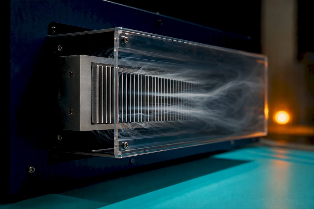
CFD earns its place in heat sink design by quantifying thermal resistance and pressure drop before you cut metal, letting you run parametric sweeps in software instead of the shop. The right sequence matters more than the tool: define your system flow and pressure-drop budget first, optimize fin geometry second, and finish with a conjugate-heat-transfer-verified model checked against a physical prototype.
TL;DR:
CFD is essential when heat sink geometries are irregular, flow is mixed, or hot spots and recirculation zones cannot be predicted analytically.
Accurate setup involves simplifying geometry with symmetry, resolving the boundary layer with proper meshing, and applying conjugate heat transfer for non-uniform heat sources.
Thermal resistance and pressure drop outputs directly inform junction temperature estimates and fan requirements, with Nusselt number useful for design comparison.
Use semi-analytical models for early screening, but verify final designs with mesh-independent CFD results to avoid costly errors.
Prioritizing flow and pressure-budget verification before geometry optimization leads to more realistic and manufacturable heat sink designs.
Table of Contents
What Is Heat Sink CFD and When Do You Actually Need It?
Closed-form correlations get you 80% of the way for a plate-fin extrusion in known crossflow. CFD earns its computational cost when geometry gets irregular, flow is mixed or impinging, or you need to see where hot spots and recirculation zones actually sit rather than assume they don’t exist. If you’re benchmarking a pin-fin array against a known Nusselt correlation, hand calculations might be enough. If you’re chasing 15% more thermal performance out of a fixed volume envelope, CFD modeling is where that margin gets found.
Heat sinks fall into a handful of geometric families, and each one carries its own thermal-versus-pressure-drop trade-off:
Plate-fin: straightforward, low pressure drop, best for ducted crossflow with moderate power density.
Pin-fin: better for omni-directional or impinging flow, adds wake turbulence that boosts local heat transfer at the cost of higher ΔP.
Microchannel: extreme surface-area density for high-flux electronics, but pressure drop rises fast as channel width shrinks.
Impingement: a jet aimed at the fin base, delivering very high local heat transfer coefficients directly under the nozzle.
Porous/lattice: metal foam or additively manufactured lattice structures that trade predictable flow paths for surface area, often needing a permeability-based CFD model rather than resolved geometry.
The core tension never disappears: more fin surface area lowers thermal resistance and raises pressure drop, and every geometry family sits somewhere different on that curve. Pin-fin designs in particular reward CFD because their wake interactions are hard to capture analytically.
Setting Up a CFD Model That Gives You Trustworthy Numbers
A heat sink CFD model is only as good as the simplifications you choose, and most bad results trace back to a shortcut in geometry, mesh, or boundary conditions rather than the solver itself.
Geometry. Exploit symmetry wherever the flow and thermal load are symmetric. A repeating fin array often reduces to a single unit cell with periodic boundaries, cutting cell count by an order of magnitude. Model the full assembly only when you suspect edge effects, bypass flow around the heat sink, or asymmetric inlet conditions from a fan or duct.
Meshing. Resolve the boundary layer with enough prism layers to capture the velocity and thermal gradients near fin walls. A poor first-cell height near a wall wrecks your convective heat transfer coefficient no matter how fine the rest of the domain is. Keep cell aspect ratios reasonable in narrow channels and near fin tips, where the flow accelerates and separates. Over-coarsened tip regions are the single most common cause of underpredicted pressure drop in heat sink CFD.
Physics. Run full conjugate heat transfer when the solid conduction path meaningfully affects the local temperature field, which is nearly always true for heat sinks with non-uniform heat sources. Fluid-only domains with convective boundary conditions can work for quick fan-curve screening but will miss fin-tip temperature drop. For turbulence, SST k-omega handles the separated, adverse-pressure-gradient flow typical of fin arrays better than a standard k-epsilon model. Laminar solutions are valid and cheaper for low-Reynolds-number microchannel flow, but check your Reynolds number before assuming it.
Boundary conditions. Specify inlet as a velocity profile when you know the fan’s delivered flow, or as total pressure when you’re solving for the operating point against a fan curve. Apply thermal loads as a mapped heat flux from a chip’s known hotspot map rather than a single lumped power value whenever you have that data. Wall treatments should match your turbulence model’s near-wall assumptions, or your y+ values will quietly invalidate the whole boundary layer.
Simplify geometry using symmetry or a repeating unit cell.
Mesh the boundary layer first, then refine tips and narrow gaps.
Choose conjugate heat transfer for anything with a non-uniform heat source.
Set inlet/outlet type based on whether flow or pressure is known.
Map thermal loads realistically instead of lumping power.
Pro Tip: Run your first pass on a coarse mesh with rough boundary conditions just to catch geometry errors and check flow direction. Debugging a broken model at high resolution wastes hours you’ll never get back.
What Do Rth, Nusselt Number, and ΔP Actually Tell You?
Thermal resistance in °C per watt is the number that translates directly into a junction temperature: multiply Rth by the dissipated power and add the inlet air temperature, and you have your worst-case junction estimate. If your CFD model reports an Rth of 0.8°C/W at 40 watts with 35°C inlet air, that chip runs at 67°C, and you know immediately whether you have margin against a 100°C limit.
Pressure drop comes out of the solver in Pascals, and fan curves are almost always published in inches of water. 1 Pa equals roughly 0.00401 in. H2O, so a heat sink showing 120 Pa of pressure drop needs about 0.48 in. H2O of static pressure from the fan at that flow rate. Skip this conversion and you’ll pick a fan that can’t actually push the air your simulation assumed.
Nusselt number is less useful as a standalone deliverable and more useful as a comparison tool: it strips out geometry scale so you can judge whether one fin design transfers heat more efficiently than another, independent of surface area.
Metric | Units | What it tells you |
Thermal resistance (Rth) | °C/W | Converts directly to junction temperature at a given power |
Junction temperature | °C | Pass/fail against the component’s rated maximum |
Nusselt number | dimensionless | Local or average heat transfer efficiency, geometry-independent |
Pressure drop (ΔP) | Pa (convert to in. H2O for fan specs) | Determines whether your fan can deliver assumed flow |
Contour plots and streamlines do the diagnostic work numbers alone can’t. A hot streak running down one side of the base almost always means bypass flow slipping around the fin array instead of through it. Recirculation zones behind thick fins show up as low-velocity pockets in a streamline plot well before they show up as a bad Rth number, giving you a head start on redesign.
Do Pressure-Drop Correlations Still Matter When You Have CFD?
They matter more, not less, because a correlation gives you a fast sanity check on whether your CFD result is even in the right neighborhood. A plate-fin pressure-drop correlation run in a spreadsheet takes seconds; if your CFD model comes back 3x higher or lower than that estimate, you’ve likely got a mesh or boundary condition problem worth chasing before you trust the detailed result.
Semi-analytical models for microchannel heat sinks with slip-flow boundary conditions run about 92% accurate against detailed CFD, making them genuinely useful for early design iterations rather than just a rough check.
A related developing-flow model for microchannel plate-fin geometries predicts pressure drop within roughly 5% for practical configurations, particularly where entrance effects dominate short channels.
Entrance and exit loss coefficients, commonly labeled Kc and Ke, account for the sudden contraction and expansion as air enters and leaves the fin channels. These losses often dominate total ΔP in short heat sinks, where the channel itself is too brief to develop meaningful friction loss.
Semi-analytical accuracy in the 90 percent range is a strong signal for early-stage screening, not a replacement for CFD verification on your final geometry.
Once you have a ΔP versus flow-rate curve from either method, plot it against the fan’s published performance curve. The intersection point is your real operating flow rate, not the flow rate stamped on the fan’s datasheet at zero back-pressure. Designing to a known flow and pressure-drop target before you optimize fin geometry avoids the common trap of building a thermally excellent heat sink that no commercially available fan can actually drive.
How Do You Run a Design Optimization Workflow?
Optimization only works when you frame it as a constrained problem, not a wish list. The standard framing: minimize thermal resistance subject to pressure drop staying under your fan-defined budget, and subject to the part fitting inside a fixed envelope.
The parameters worth sweeping, roughly in order of impact for most fin-array designs:
Fin height, since it drives both surface area and flow blockage simultaneously.
Fin spacing, which trades channel count against per-channel velocity and friction loss.
Fin thickness, mostly a manufacturability and fin-efficiency lever rather than a big thermal one.
Base thickness, which matters most when the heat source is small and spreading resistance dominates.
Inlet or nozzle location, critical for impingement and ducted designs where bypass flow is a risk.
Running dozens of full CFD cases across five parameters gets expensive fast, which is where surrogate modeling earns its keep. Sample a modest set of CFD runs across your parameter space, then fit a surrogate, generalized polynomial chaos and neural network surrogates are both common choices, to predict Rth and ΔP for combinations you haven’t directly simulated. Transfer learning approaches have cut surrogate training time by roughly 5x in published examples, which matters when you’re iterating on a tight development schedule.
Pro Tip: Build your Pareto front (Rth versus ΔP) from the surrogate first, then run full CFD only on the two or three candidate points that actually sit on the efficient frontier. Verifying ten points instead of two hundred is the entire point of the surrogate step.
A Heat Exchanger Optimization workflow follows this same sample, build, optimize, verify sequence, and it generalizes well beyond heat exchangers to any fin-array optimization problem.
Where Do Advanced CFD Techniques Actually Pay Off?
Conjugate heat transfer solvers can struggle with numerical stiffness when solid and fluid domains have wildly different conductivities, copper against air is a factor of roughly 15,000. That contrast can produce oscillatory divergence in a fully coupled solve.
The hFTB approach (heat transfer coefficient forward, temperature backward) breaks the coupling into a one-way iterative exchange instead of solving both domains simultaneously, which stabilizes convergence on high-conductivity-ratio problems that otherwise stall.
Under-relaxation on the coupled boundary is a simpler, older fix for the same stiffness, trading iteration count for stability.
Microchannel flows at small enough scales enter the slip-flow regime, where the modified Knudsen number tells you whether standard no-slip wall assumptions still hold. Below a certain channel dimension, ignoring slip-flow physics produces a pressure-drop error that grows as channels shrink.
Surrogate acceleration keeps expanding beyond basic polynomial chaos. Neural network surrogates trained with transfer learning can reuse knowledge from one geometry family to speed up training on a related one, trading a small accuracy hit for a large speed gain during early exploration.
None of this replaces a converged, properly meshed CFD run for your final design. It changes how many of those runs you need and how fast you get through the ones that matter.
How Do You Know Your CFD Results Are Right?
Mesh independence isn’t optional, and skipping it is the fastest way to publish a wrong Rth number with total confidence. Run the same case at three mesh densities and track how maximum temperature and pressure drop change between them.
Start with a mesh you expect is too coarse and one you expect is fine, then add a middle density.
Compare max temperature and ΔP across all three; a common acceptance target is under 2 to 3% change between the two finest meshes.
If results haven’t converged, refine further, particularly near walls, fin tips, and any separation point.
Only trust the result once the finest practical mesh shows negligible change from the next-coarser one.
Validating against a physical prototype means measuring ΔP and Tmax at instrumented points that match where your CFD reports them, not wherever a thermocouple happened to fit. Report measurement uncertainty alongside the value.
When CFD and test data disagree, the usual suspects are bypass flow the model didn’t capture, boundary conditions that assumed a cleaner inlet than the real duct provides, or fixed material properties standing in for the temperature-dependent conductivity aluminum and copper actually exhibit.
Guides and Tools for Executing These Workflows
For worked examples that go deeper into specific geometries, Jewlztech’s heat sink design guide and CFD heat transfer solver mapping walk through governing equations and setup decisions in more detail than fits here. The Jewlztech toolkit supports conjugate heat transfer setup, parametric sweeps across fin geometry, and a built-in material property database with temperature-dependent values, mapping directly onto the workflow described above.
Should You Run Transient or Steady-State Simulations?
Steady-state simulation is the right default for continuous-duty heat sinks: constant power dissipation, constant airflow, and a design question that’s really “what’s the equilibrium Rth.” It converges faster and gives you a clean number to compare against a spec limit.
Transient simulation earns its added cost when power cycles, fan speed ramps, or you care about how fast a component reaches a thermal limit after a load step. A CPU under bursty compute load, a power module switching on and off, or a system with a fan that spins up gradually all behave differently in a transient run than a steady-state one would predict. Steady-state analysis on a cyclic load simply reports the wrong number, usually optimistic, because it can’t capture the temperature overshoot during the worst part of the cycle.
Thermal mass matters here. A heat sink with high thermal mass smooths out short power transients, and a transient CFD run is the only way to quantify how much smoothing you actually get before deciding you can rely on it rather than sizing for the instantaneous peak.
The practical rule: use steady-state for baseline geometry screening and fan selection, where speed matters and duty cycle is constant. Switch to transient once you’re validating a specific application with known duty cycle data, especially anything with pulsed power electronics or intermittent high-performance computing loads. Running every design iteration as transient wastes compute time you don’t need to spend; running your final validation case as steady-state when the real application is bursty is the more expensive mistake.
How Do You Model Thermal Interface Materials in CFD?
The thermal interface material sitting between chip and heat sink base is often the largest single contributor to total thermal resistance in a well-designed system, and it’s also the easiest thing to model wrong. A TIM layer is thin, usually well under a millimeter, and meshing it as resolved solid geometry forces an extremely fine mesh in a tiny region just to keep cell aspect ratios sane.
The common shortcut is a thermal contact resistance boundary condition applied at the interface instead of a meshed solid layer. You specify a resistance value in °C·cm²/W or equivalent units, sourced from the TIM manufacturer’s datasheet, and the solver applies it as a temperature jump across that surface without needing to mesh the material itself.
The catch is that datasheet TIM values are usually measured under a specific clamping pressure and bond-line thickness, and real assembly pressure rarely matches that test condition exactly. A TIM specified at 50 microns bond-line thickness that actually assembles at 80 microns due to an uneven mounting surface can add measurably more resistance than the simulation assumed. If your CFD-predicted junction temperature runs consistently below what you measure on a prototype, an underestimated TIM resistance is one of the first places to check, right alongside bypass flow and boundary condition mismatches.
For high-power designs where the TIM layer contributes a meaningful share of total Rth, it’s worth running the model at both the datasheet-nominal resistance and a worst-case bond-line thickness to see how sensitive your final junction temperature actually is to assembly variation.
How Do You Visualize CFD Results to Find Design Flaws?
Raw numbers tell you whether a design passes or fails. Visualization tells you why, and where to fix it.
Velocity contour slices through the fin channels are the first thing worth checking, because they reveal bypass flow immediately: air skirting around the outside of the fin array instead of through it shows up as a fast-moving region outside the intended flow path and a comparatively stagnant one inside it. That single image often explains a disappointing Rth number faster than any amount of number-crunching.
Streamlines add the trajectory information a static contour can’t show. Recirculation zones behind thick fins or downstream of an abrupt cross-section change appear as closed loops or tight spirals in a streamline plot, and those zones are dead thermal weight, occupying volume without moving heat efficiently.
Temperature contours on the fin surfaces and base plate show gradient patterns that point directly at spreading resistance problems. A base plate that’s noticeably hotter directly under the chip than at its edges tells you the base is too thin, or the material’s conductivity is lower than the design assumed.
Wall shear stress plots are underused but genuinely useful. High shear correlates with high local convective heat transfer, so a shear plot often mirrors the areas doing the most thermal work, letting you check whether that work lines up with the areas that actually run hot.
Pro Tip: Overlay a temperature contour and a streamline plot on the same view rather than switching between two separate images. The correlation between a hot spot and a nearby recirculation zone is often invisible until you see both at once.
Where the Conventional Advice Falls Short
Most heat sink CFD content treats geometry optimization as step one and flow delivery as an afterthought, tuned once the “ideal” fin array is already locked in. That ordering produces beautifully efficient designs that no fan on the market can actually drive at the assumed flow rate. The research on pressure-drop-target design backs a different sequence, and it’s the one worth defending: pin your flow and pressure-drop budget against a real fan curve before you touch fin spacing.
What’s overrated is chasing a lower Rth number in isolation. A heat sink that shaves another 0.1°C/W off thermal resistance while doubling pressure drop is usually a worse engineering outcome, not a better one, because it forces a louder, more expensive, or entirely different fan into the bill of materials. Semi-analytical correlations running at 90+ percent accuracy against full CFD deserve more trust for early screening than most engineers give them; running full CFD on every candidate geometry before narrowing the field wastes compute budget that surrogate methods exist specifically to save.
What the reader should prioritize first is unglamorous: get the flow budget right, verify with a mesh-independent CFD model, and only then chase fin geometry refinement.
— Joel
Get Started with Jewlztech’s Thermal Simulation Toolkit
If you’ve been sketching Rth and ΔP estimates by hand or waiting on a CFD consultant’s turnaround, Jewlztech’s toolkit puts the full workflow described above directly in your hands: conjugate heat transfer setup, parametric fin-geometry sweeps, and a built-in temperature-dependent material property database that removes the guesswork of picking aluminum versus copper properties at the wrong operating temperature.

Start small. Run a single-case Rth and ΔP study on a geometry you already have drawings for, and compare the output against a hand-calculated correlation before trusting a full parametric sweep. The free tier of the engineering toolkit is built for exactly that kind of first pass, and it’s a low-risk way to see whether the workflow fits how your team actually works before committing to the paid subscription tier. When you’re ready for full parametric optimization and surrogate-assisted design exploration, the CFD simulation software page walks through the premium Thermalysis Toolkit features that support it. Try a case this week, and see what your current design’s real pressure-drop budget actually looks like.
Sources
Recommended
Comments