
CFD Heat Transfer: Mapping Governing Equations to Solver Setup

Updated: Sep 16

CFD heat transfer couples conduction, convection, and radiation with a fluid dynamics solution to predict temperature distribution, heat flux, and hot spots across a design. Engineers use those outputs to size heat sinks, validate heat exchanger performance, and check where thermal loads exceed material limits. The three most common applications are electronics cooling, heat exchanger design, and aerodynamic heating on high-speed vehicles.
TL;DR:
An accurate CFD heat transfer simulation requires proper modeling of conduction, convection, and radiation, especially at high surface temperatures or complex geometries.
The choice of energy equation formulation impacts the handling of compressibility, viscous heating, and species transport, with total energy and enthalpy forms suited for high-speed and reacting flows.
Coupling strategies for conjugate heat transfer range from fully coupled for small, tight geometries to loosely coupled for slower-responding solids, with time-step adjustments critical for accuracy.
A staged setup process, including mesh refinement near walls and validation against benchmarks, is essential to prevent convergence issues and ensure fidelity to actual behavior.
Validation against simple benchmark cases and careful physics modeling often outweigh the importance of turbulence model choice for producing reliable thermal CFD results.
Table of Contents
How Do the Three Modes of Heat Transfer Work in CFD?
Every thermal CFD model juggles three physical mechanisms at once, and getting the balance wrong is the most common reason simulations disagree with test data.
Conduction happens inside solids, and its accuracy depends on how well you capture thermal conductivity, including anisotropic behavior in materials like PCB laminates or composite skins. A thin wall (a heat sink fin, a can wall) can often be modeled with a shell conduction approximation instead of a fully meshed solid, saving cells without sacrificing much fidelity.
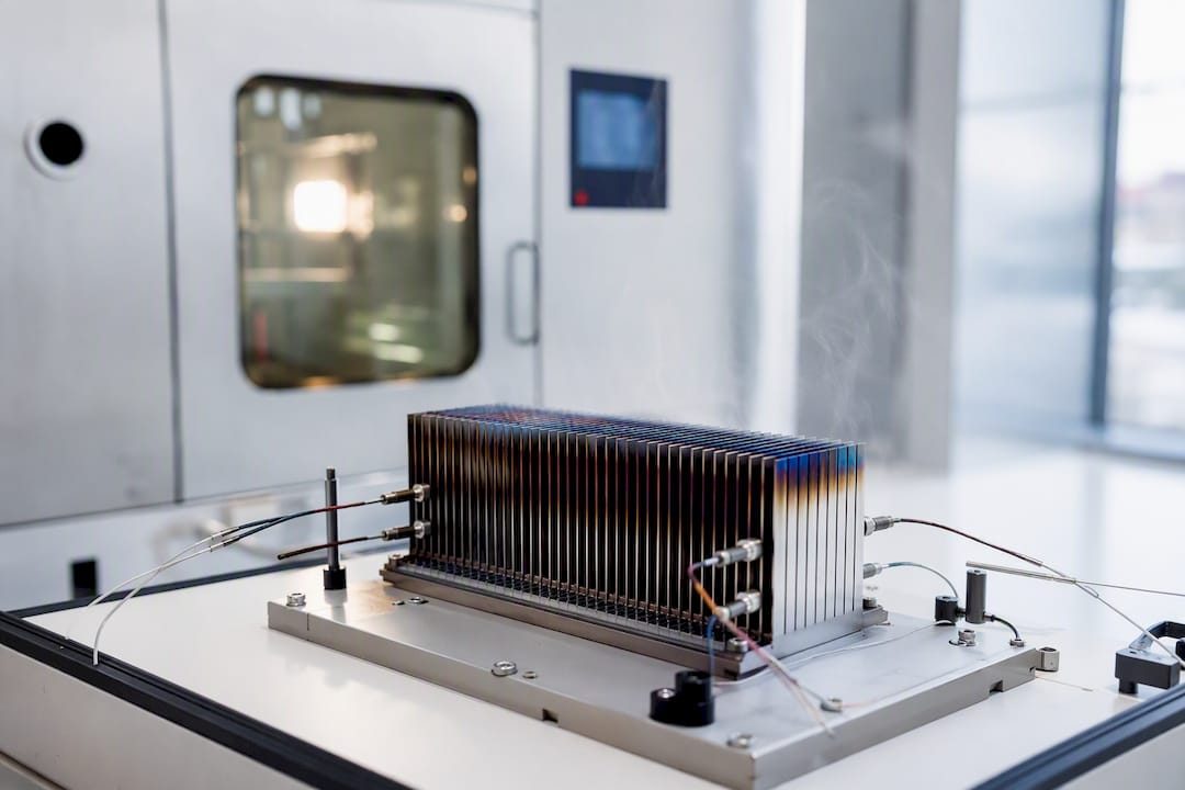
Convection is where the fluid solution and the thermal solution actually meet. Boundary-layer resolution controls how well you predict the wall heat-transfer coefficient, and the natural-versus-forced convection regime changes which turbulence model and mesh density you need near the wall.
Radiation matters more than most engineers assume once surface temperatures climb past a few hundred degrees Celsius, or when surfaces face each other across a gap, like inside an oven or a satellite bay. Surface-to-surface radiation models handle most enclosure problems; participating-media models are needed only when the fluid itself absorbs or emits significant radiant energy, like combustion gases.
Modeling implications compound quickly:
Treat conductivity, specific heat, and density as temperature-dependent for any run spanning more than about 50°C, not as constants.
Decide early whether thin-wall (shell) conduction is acceptable or whether the wall needs full mesh resolution.
Include radiation once surface temperature or view-factor geometry makes it comparable in magnitude to convection.
Match your turbulence and near-wall treatment to how much boundary-layer detail the heat-transfer coefficient actually needs.
What Energy Equation Form Should You Solve?
The energy conservation equation is the backbone of every thermal CFD run, and most solvers give you at least three ways to write it: total energy, internal energy, and enthalpy. The choice is not cosmetic. It changes how the solver handles compressibility, viscous heating, and species transport.
Total energy formulations are standard for compressible, high-speed flow where kinetic energy exchanges matter, like aerodynamic heating on a reentry vehicle. Enthalpy-based forms, widely used for ideal-gas and combustion problems, simplify the pressure-work terms and tend to be more numerically stable for reacting flows. Internal energy forms show up in low-Mach incompressible solvers where kinetic-energy coupling is negligible.
Watch for these energy-source terms before you trust a result:
Viscous dissipation, which is usually negligible below Mach 0.3 but adds real heat in high-shear or high-speed flows.
Volumetric heat sources like Joule heating in electronics or chemical reaction heat release.
Species enthalpy transport in multi-component or combusting flows.
Pro Tip: For many low-Mach engineering problems, viscous dissipation adds nonlinearity without adding accuracy — turn it off unless you have a specific reason to keep it.
What Is Conjugate Heat Transfer and How Do You Couple It?
Conjugate heat transfer, or CHT, solves the solid conduction and fluid convection domains together so heat can flow naturally across the interface without an assumed heat-transfer coefficient. Typical cases include electronics enclosures, engine components, and heat exchanger tube walls where the wall temperature itself is unknown and part of what you’re solving for.
Two coupling strategies dominate practice:
Fully coupled solves fluid and solid equations simultaneously each iteration, giving the tightest accuracy but the highest computational cost, and it’s the right call for small, tightly coupled geometries.
Loosely coupled (staggered) solves fluid and solid domains separately and exchanges boundary data at intervals, which cuts cost substantially when the solid responds much slower than the fluid.
Interface treatment typically uses Dirichlet–Neumann coupling: one side gets a temperature boundary condition, the other gets a heat-flux condition, and the solver iterates until both agree.
Time stepping needs attention too. A thin electronics enclosure wall reacts quickly, while a thick pressure vessel wall takes considerably longer to reach thermal equilibrium. Give the solid a larger time step than the fluid whenever that mismatch is significant, a strategy detailed in Jewlztech’s conjugate heat transfer simulation guide.
How Do You Set Up a Thermal CFD Model Correctly?
A clean setup sequence prevents most of the convergence headaches that show up later. Work through it in this order:
Define boundary conditions on every wall and interface: fixed temperature, fixed heat flux, or convective (heat-transfer coefficient plus ambient temperature) depending on what data you actually have.
Assign material properties as functions of temperature, not single values, especially thermal conductivity, specific heat, and density for anything crossing a wide temperature range.
Choose a turbulence model based on the flow regime, and check near-wall y+ before trusting the heat-transfer coefficient: wall functions handle y+ around 30 to 300, while a fully resolved boundary layer needs y+ near 1.
Mesh solids and fluids with different priorities: solids need enough layers through the thickness to resolve the temperature gradient, while fluid domains need boundary-layer inflation to capture the thermal boundary layer.
Set solver controls: use under-relaxation on the energy equation during early iterations, initialize with a reasonable temperature field rather than zero, and pick a transient time step based on the fastest thermal response you’re resolving.
A few things trip up even experienced users:
Skipping radiation on high-temperature enclosures because it “seemed convective” undercuts accuracy without warning.
Leaving default residual targets too loose for the energy equation, which converges more slowly than momentum and continuity.
Using a coarse mesh in the thermal boundary layer while a fine mesh handles the velocity boundary layer, so the heat-transfer coefficient is under-resolved even though the flow field looks fine.
Pro Tip: Solve momentum and continuity for a few hundred iterations before turning on the energy equation — a converged flow field makes the thermal solve far more stable. For a deeper walkthrough of inlet, outlet, and wall boundary options, see Jewlztech’s CFD boundary conditions guide.
Why Do Thermal CFD Models Fail to Converge or Match Reality?
Most bad thermal CFD results trace back to a handful of repeat offenders: a physics term left on (or off) by mistake, a mesh too coarse near the wall, a boundary condition borrowed from a datasheet that doesn’t match actual operating conditions, or unnecessary viscous dissipation adding numerical stiffness to a low-speed problem.
Fixing convergence usually means staging complexity rather than throwing every physics model in from iteration one:
Start with flow only, add energy, then add radiation and turbulence refinements in sequence.
Increase mesh resolution near walls specifically, not just globally, since boundary-layer resolution drives heat-transfer coefficient accuracy.
Run a grid-convergence study with at least three mesh densities before trusting a single result.
Validation should follow a similar staged logic. Compare against a canonical benchmark first, like a heated flat plate or a driven cavity with known heat flux, since these give the fastest confidence check before trusting a complex CHT model. Then compare against thermal-camera or thermocouple data from the actual hardware. If results still diverge by a wide margin after mesh refinement, that’s the signal to escalate to physical testing rather than keep tuning the model.
Pro Tip: A single consumer-grade evidence-grading tool or quick simulation is not a substitute for benchmark validation on safety-critical thermal designs — treat early results as directional until checked against a known case.
Which Applications Demand Different Thermal CFD Priorities?
Electronics cooling, heat exchanger design, and aerospace heating each push a thermal model in a different direction, and treating them the same way wastes compute time or accuracy.
Electronics: resolving conduction paths through PCB copper layers matters more than fluid turbulence detail; transient thermal response during power cycling often matters more than steady-state peak temperature. See Jewlztech’s PCB thermal analysis workflow for a full setup sequence, and the active versus passive cooling guide for choosing a cooling strategy.
Heat exchangers: fluid selection, including additives like nanofluids, trades heat-transfer enhancement against pressure drop. One shell-and-tube study found significantly higher heat transfer at high nanoparticle loading, but with pressure drop also increasing substantially, which pushed the net performance benefit toward lower particle concentrations.
Aerospace: compressibility and shock heating demand total-energy formulations and fine surface meshing to capture heat flux accurately at high Mach numbers.
Steady-state analysis suits equilibrium performance checks; transient analysis is required whenever power cycling, startup, or a rapidly changing flight condition drives the design.
Where Can Engineers Find Practical Tools and Guides?
Jewlztech’s engineering toolkit, Thermalysis, is a web-based engineering application for conduction, convection, and radiation analysis, with a built-in material property database and temperature-dependent inputs. It provides engineers with a fast way to perform thermal calculations and sanity checks before committing to a full CFD simulation. Pair it with Jewlztech’s heat transfer model guide for the underlying mathematics and the conjugate heat transfer guide for coupling strategy.
What Actually Separates a Good Thermal CFD Model From a Bad One?
Most of the advice circulating about thermal CFD focuses on turbulence models, as if picking the right RANS variant is the hard part. It usually isn’t. The bigger failure mode is treating the energy equation as an afterthought, bolted onto a converged flow solution instead of built into the setup from the start. A model with a mediocre turbulence choice but correct temperature-dependent material properties and a sane radiation treatment will usually beat a model with a perfect turbulence setup and constant properties.
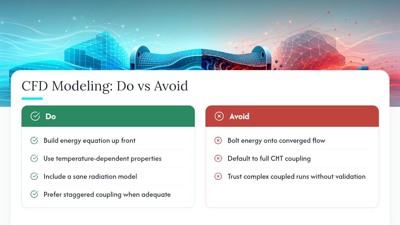
The other place conventional advice falls short is coupling strategy. Engineers default to fully coupled CHT because it sounds more rigorous, then wait hours for a result a staggered, loosely coupled run could have delivered in a fraction of the time with nearly identical accuracy. Reserve full coupling for genuinely tight thermal interactions, not as a default setting.
If you take one thing from this guide, prioritize validation against a canonical benchmark before you trust a complex coupled result. A heated flat plate case costs you twenty minutes; a wrong hot-spot prediction on a production board costs a redesign.
— Joel
Get Thermal Analysis Right the First Time
Jewlztech built its engineering toolkit for exactly the workflow this guide walks through: checking conduction, convection, and radiation by hand before committing to a full CFD study, without needing a separate license or a steep learning curve to get a credible number.

The Thermalysis Toolkit is a web-based engineering application that supports variable material properties across a wide temperature range, includes a built-in material property database, and brings multiple heat-transfer modes into one integrated environment. It is suited to engineers who need a fast thermal sanity check alongside a CFD analysis rather than a second full simulation environment. Engineers moving from hand calculations into coupled-physics work can pair Thermalysis with Jewlztech’s CFD simulation software for fluid-solid problems, including conjugate heat transfer and heat exchanger analysis. Use the web-based toolkit to evaluate your next thermal problem against a benchmark case before committing significant time to a full CHT setup.
Sources
Recommended
Comments