
Engineers: Use Bi ≤0.1 and Fo >0.2 for Transient Heat Conduction

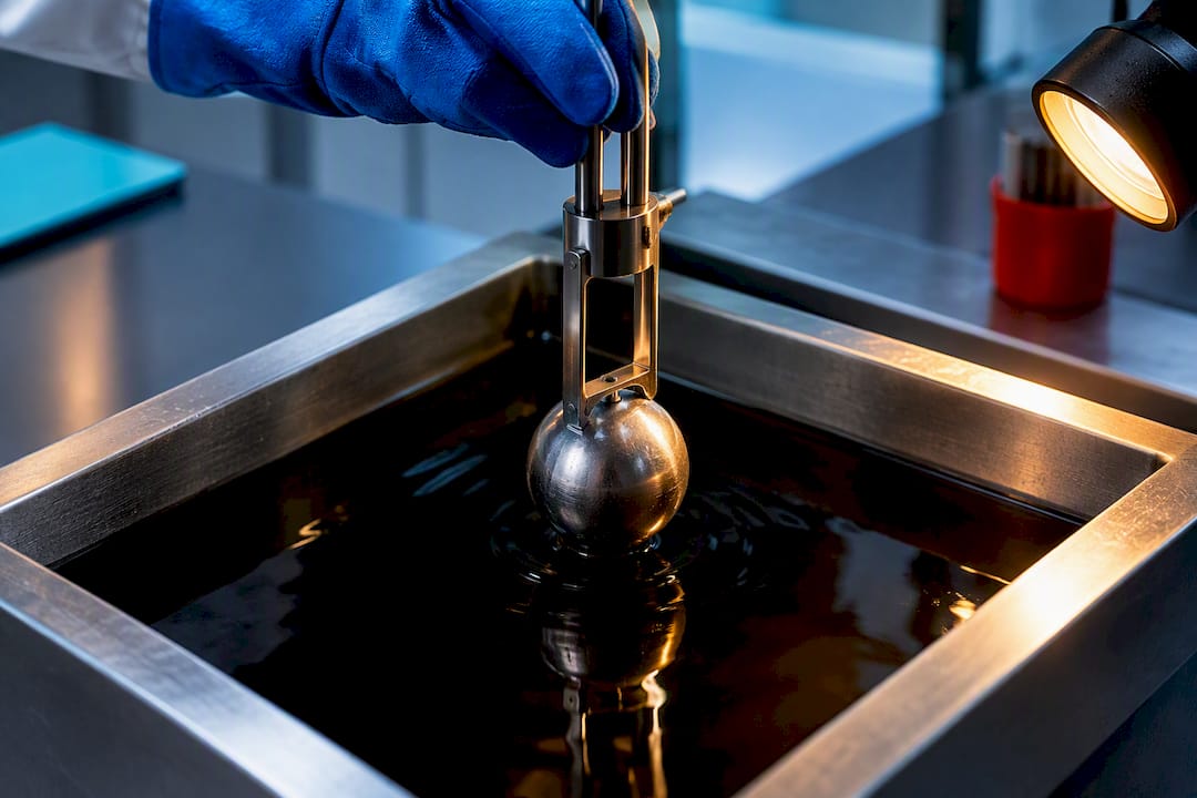
Transient heat conduction is the time-dependent temperature response inside a solid, governed by the diffusion form of the heat equation rather than a fixed steady profile. It shows up whenever a part heats or cools faster than it can equalize internally: quenching, engine startup, a PCB under a load spike, a turbine blade at ignition. The fast way to know which solution method you need is to check two numbers, the Biot number and the Fourier number, before you touch a differential equation.
TL;DR:
If the Biot number is less than or equal to 0.1, lumped capacitance models apply, simplifying the analysis to an exponential decay based on the thermal time constant.
For geometries where Bi exceeds 0.1, spatial solutions involving eigenfunctions or semi-infinite models are necessary, with the series converging quickly once Fourier number surpasses 0.2.
Using appropriate characteristic length—volume divided by surface area—prevents misclassification of thermal behavior and is essential for accurate estimation.
Radiation becomes significant at surface temperatures in the hundreds of degrees, and models that neglect it may underestimate cooling rates at high temperatures.
Numerical simulations are required when boundary conditions change over time, material properties depend on temperature, or the object has multilayered structures, making analytical methods insufficient.
Table of Contents
What Is the Transient Heat Conduction Equation?
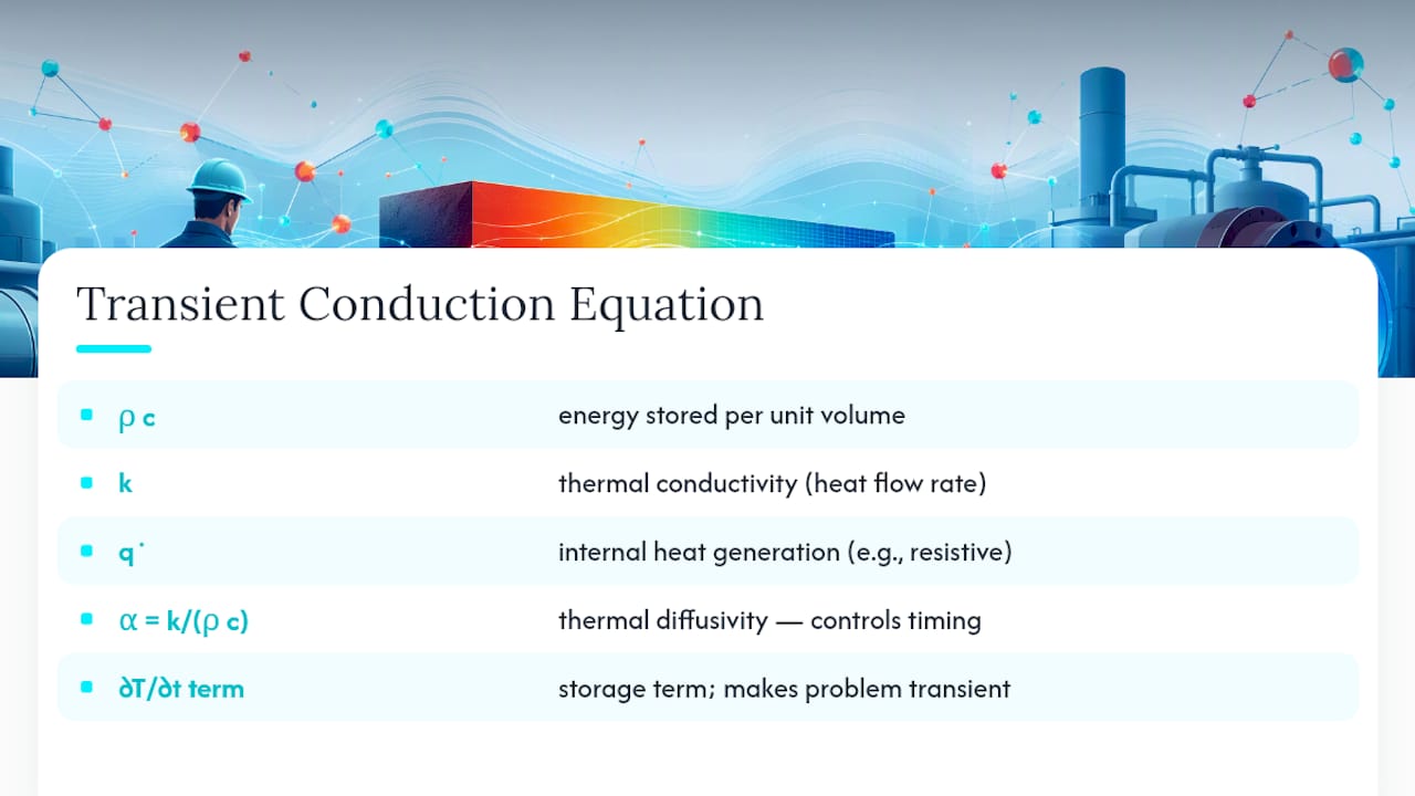
The governing relationship for unsteady heat transfer is $\rho c \frac{\partial T}{\partial t} = abla \cdot (k abla T) + \dot{q}$. Density ($\rho$) and specific heat ($c$) set how much energy a material stores per degree; thermal conductivity ($k$) sets how fast heat moves through it; $\dot{q}$ is any internal heat generation, like resistive heating in a circuit board. The left side, the storage term, is what makes the problem transient. Drop it and $\partial T/\partial t$ goes to zero, and you’re back to plain steady-state conduction.
The ratio that actually controls timing is thermal diffusivity, $\alpha = k/(\rho c)$. It’s not conductivity alone that determines how fast a temperature front moves through a solid. A dense, high heat capacity metal can have decent conductivity yet still respond sluggishly because it takes more energy to shift its temperature. Diffusivity is the number that reconciles those two effects, and it’s what defines the transient conduction equation’s time scale.
Steady-state conduction gives you one temperature field, forever. Transient conduction gives you a whole history, $T(x,t)$, which is exactly what you need if you’re controlling a quench rate or predicting when a component crosses a failure temperature.
Lumped Capacitance and the Biot Number Test
Skip the spatial math entirely when a part’s internal resistance to conduction is small next to its surface resistance to convection. That’s the entire premise behind the lumped capacitance method, and it turns a partial differential equation into an energy balance you can solve by hand: $mc\frac{dT}{dt} = hA(T_\infty - T)$. Integrate that and you get a clean exponential decay:
$$T(t) = T_\infty + (T_i - T_\infty)e^{-t/\tau}$$
The gatekeeper is the Biot number, $Bi = hL_c/k$, where $L_c$ is the characteristic length (usually volume divided by surface area, $V/A$, not the radius or thickness people default to). The standard applicability rule is Bi ≤ 0.1, because below that threshold the temperature gradient inside the part is small enough to ignore without meaningful error.
Three steps get you a working answer fast:
Compute $Bi = hL_c/k$ using $L_c = V/A$.
If $Bi \le 0.1$, calculate the thermal time constant $\tau = \rho V c/(hA)$.
Plug $\tau$ into the decay equation to find the time needed to hit a target temperature.
Pro Tip: A 2 cm steel ball in still air often looks lumpable at first glance, but check Bi with the real convection coefficient for air, not the value you’d use for a water quench. Air’s low h can push Bi well under 0.1 even for parts that would fail the test in liquid.
Solving Slabs, Cylinders, Spheres, and Semi-Infinite Solids
Once Bi climbs past 0.1, you need a solution that accounts for spatial gradients, and the geometry of the part decides which one. Finite shapes (a plate, a rod, a ball) get infinite-series solutions built from eigenfunctions and eigenvalues specific to that geometry. Deep or thick bodies exposed briefly get semi-infinite solid solutions instead, built around the error function rather than a series.
Slab geometry fits thin plates and flat stock where conduction dominates through the thickness.
Cylinder geometry fits long rods, pipes, and shafts where radial conduction matters most.
Sphere geometry fits compact rounded parts like ball bearings or pellets.
Semi-infinite solid solutions fit surface quenching, flash heating, or any case where the far side of the material never feels the temperature change during the time window you care about.
The series solutions converge fast enough that a single leading term is usually sufficient once $Fo > 0.2$, which is the practical cutoff most references use before recommending full series expansion instead. Below that, you need more terms or a numerical approach, because the early-time response is dominated by higher-order modes the first term can’t capture.
Using Fourier Number and Heisler Charts for Fast Answers
The Fourier number, $Fo = \alpha t / L_c^2$, is time rescaled by how fast heat diffuses through the part’s characteristic length. A low Fo means the temperature change is still confined near the surface; a high Fo means the whole part has started responding together.
Heisler and Gurney-Lurie charts turn that dimensionless pairing into a lookup problem instead of a calculus problem. Three chart types matter:
One gives dimensionless center temperature versus Fo for a given Bi.
A second gives the temperature ratio at any position relative to the center.
A third gives total heat transferred, useful for energy accounting in a quench or heat treatment cycle.
First-term approximations built into these charts hold well once Fo exceeds roughly 0.2. Below that, interpolate carefully between chart curves or fall back on the full series, since chart reading error compounds fast at low Fo.
When Analytic Shortcuts Break Down
Lumped models, series solutions, and Heisler charts all assume constant properties and simple, unchanging boundary conditions. Real processes rarely cooperate. Time-varying convection coefficients during a quench, temperature-dependent conductivity in a casting, and multilayer composites with different properties per layer all defeat the standard separation-of-variables approach, which is exactly why specialized shifting-function techniques exist for time-dependent heat transfer coefficient problems, and why most engineers reach for numerical simulation instead.
Two time-stepping choices dominate finite element and finite volume solvers. Explicit schemes are cheap per step but stability forces very small time steps tied to mesh size. Implicit schemes, including Crank-Nicolson, cost more per step but stay stable at much larger time steps, which is why most transient thermal analysis defaults to implicit integration.
A short setup checklist keeps results trustworthy:
Refine the mesh near boundaries where gradients concentrate.
Size the time step using Fo, not an arbitrary round number.
Add radiation once surface temperatures climb into the several-hundred-degree range.
Validate a coarse run against a lumped or Heisler estimate before trusting a fine mesh.
Pro Tip: Radiation losses scale with the fourth power of absolute temperature, so a model that’s fine at 80°C can quietly underestimate cooling rate once the same part sits at furnace temperature. If you dropped radiation from a low-temperature model, don’t assume it’s still safe to drop at high temperature.
Two Quick Worked Examples
Example 1, sphere cooling. A small steel sphere quenched in oil: compute $Bi = hL_c/k$ with $L_c = V/A = r/3$. If Bi comes in under 0.1, skip straight to $\tau = \rho V c/(hA)$ and solve $T(t) = T_\infty + (T_i - T_\infty)e^{-t/\tau}$ for the time to reach a target temperature. This is the Biot number criteria check in practice.
Example 2, semi-infinite surface cooling. A thick slab suddenly exposed to cold air on one face: the interior hasn’t felt the change yet, so the error-function solution applies. You need only $\alpha$, exposure time, and depth from the surface to estimate the temperature at any point.
Common applications following this exact logic: heat treatment and quenching, gas turbine startup transients, PCB thermal spikes under load, and casting solidification and cooling — all processes where reliable temperature monitoring solutions for cold chain management play a crucial role.
What Practitioners Get Wrong About Transient Conduction
The most common mistake I see isn’t picking the wrong equation, it’s picking the wrong characteristic length for Bi. Using thickness or radius instead of $V/A$ can flip a part from “lumped is fine” to “you need a spatial solution,” and most people never notice because the arithmetic still produces a number that looks reasonable.
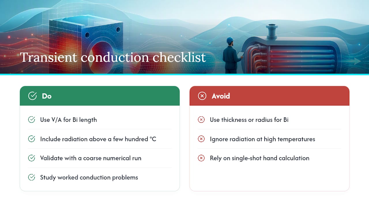
The second mistake is ignoring radiation until a part is already failing thermally in a model. If your process temperature climbs past a few hundred degrees, radiation isn’t optional anymore, and Fourier-based continuum models themselves start showing their limits at nanoscale or ultrafast time domains, though that’s a corner case most engineering work never touches.
My advice: validate every quick estimate against a coarse numerical run before you commit to a design based on a hand calculation alone, and lean on worked problems like the heat conduction calculations format to build intuition before trusting a single-shot answer.
— Joel
Run Your Own Transient Conduction Estimates With Jewlz Technologies
Jewlztech built the Engineering Toolkit around exactly the workflow this article walks through: check Bi and Fo first, then pick the right solver instead of guessing. The toolkit bundles a material property database with conduction, convection, and radiation models in one place, so you’re not hunting down $k$, $\rho$, and $c$ values from three different textbooks while your quench time calculation waits.

Basic tools, including transient solver templates and example worksheets that mirror the sphere-cooling and semi-infinite cases above, are available for free access. Engineers running production heat treatment schedules, turbine startup analysis, or multilayer composite modeling can step up to the subscription tier for the full Thermalysis Toolkit transient solver and advanced templates. Start with the free tier and try the Jewlz Engineering Toolkit on your next quenching or startup transient problem to see where your hand calculation and the numerical result start to diverge.
Sources
FAQ
What Are 5 Examples of Heat Conduction?
Common examples include a metal spoon heating up in hot soup, a frying pan transferring heat from burner to food, an ice cube cooling a drink, a soldering iron heating a circuit board, and heat moving through a building wall in winter. Most of these are transient during the initial temperature change and settle toward steady-state afterward.
What Is the Difference Between Steady-State and Transient Heat Transfer?
Steady-state heat transfer means temperature at every point stays constant over time, so the storage term in the heat equation drops out entirely. Transient, or unsteady state heat transfer, means temperature is still changing with time, which is the case during startup, shutdown, or any sudden boundary condition change.
What Are the Three Types of Heat Transfer?
The three modes are conduction, convection, and radiation. Conduction moves heat through direct contact within a solid, convection moves it through fluid motion at a surface, and radiation moves it through electromagnetic waves, which becomes significant once temperatures climb into the several-hundred-degree range, as covered in convection, conduction, and radiation examples.
What Is the Problem of Heat Conduction?
The core problem is predicting a temperature field inside a solid given its material properties, geometry, and boundary conditions, whether that field is constant (steady-state) or evolving (transient). Solving it means picking the right tool for the job: lumped capacitance for low-Bi parts, series or chart solutions for finite geometries, or numerical simulation with an implicit time-stepping scheme when boundary conditions or material properties vary with time.
How Do I Know if I Need Numerical Simulation Instead of a Hand Calculation?
You need numerical simulation once boundary conditions vary with time, material properties change significantly with temperature, or the part has multiple layers with different properties, since these conditions break the assumptions behind lumped capacitance and standard series solutions. Tools like Jewlz’s thermal analysis software handle these cases without requiring a custom solver build.
Recommended
Comments